Introduction

Symptoms and disorders

The application of network thinking to psychometric questions has led to rapid developments in several subfields of psychology, most notably clinical psychology and psychiatry. To understand why the network approach has gained traction, it is helpful to first examine how psychologists traditionally conceptualize the relationship between symptoms and disorders.

Traditional View: Latent Variable Models

In Western medicine and much of clinical psychology, a disease model has typically been applied to psychopathology. This model assumes that an underlying disorder (latent variable) causes the observable symptoms. For instance, major depressive disorder (MDD) might be conceptualized as an unobserved pathogenic factor leading to symptoms such as insomnia, fatigue, excessive worrying, and concentration problems. Here, symptoms are viewed as passive indicators of a single latent construct, meaning they covary primarily because they reflect the same root cause.

Alternative View: Network Theory

By contrast, network theory (Borsboom & Cramer, 2013) proposes that symptoms are active, interacting components of a causal system. Rather than being mere indicators of an underlying disorder, symptoms directly influence one another. For example, insomnia can precipitate fatigue, which in turn can cause concentration difficulties, creating feedback loops that sustain the disorder. According to this approach, mental disorders emerge from the structure and dynamics of these symptom networks. Targeting the most influential (or “central”) symptoms may therefore disrupt maladaptive feedback loops and lead to widespread improvements in the symptom network.

Psychopathology as Complex Networks

Building on the network perspective, researchers have increasingly recognized that psychopathologies can be viewed as complex networks of interrelated symptoms. This reconceptualization addresses several long-standing critiques of latent variable models.

Critiques of Latent Variable Models

Recent work (e.g., Lange et al., 2020) highlights three assumptions of latent variable models that may be unrealistic when applied to mental disorders:

1. Common-Cause Assumption: Latent variable models assume that a single underlying cause (the disorder) predicts all associated symptoms. In major depressive disorder (MDD), for example, a single factor might be invoked to explain persistent sadness, loss of interest, and fatigue. However, research increasingly shows that these symptoms can stem from multiple, interacting causes (e.g., negative thinking patterns, hormonal imbalances, environmental stressors).

2. Assumption of Exchangeability: Traditional models often consider symptoms as interchangeable indicators of the same underlying construct. Clinical evidence, however, suggests that individual symptoms can play unique roles. For instance, in generalized anxiety disorder (GAD), excessive worrying may trigger insomnia, which then exacerbates fatigue and concentration problems. These symptoms are not simply redundant manifestations of a latent factor; they have distinct positions in the overall clinical picture.

3. Principle of Local Independence: Latent variable theory holds that once the latent variable is statistically controlled, symptoms should not significantly correlate with one another. Yet empirical data often reveal persistent correlations among symptoms even after adjusting for the latent variable. For instance, in MDD, fatigue and concentration difficulties frequently co-occur independently of overall depression severity, indicating that symptoms may have direct causal or interactive relationships.

Advantages of the Network Approach

In response to these critiques, the network approach conceptualizes mental disorders as complex networks of interacting symptoms. This reconceptualization involves several key insights:

1. Causal Interactions Between Symptoms: Symptoms may directly trigger or amplify one another, forming positive feedback loops that sustain a disorder. For example, insomnia → fatigue → concentration problems in depression.

2. Emergence of Symptom Co-Occurrence: Symptom co-occurrence arises from network structure. Instead of a single underlying factor forcing symptoms to cluster, groups of symptoms become interconnected through reciprocal influences. These emergent clusters of symptoms are often labeled as distinct mental disorders, such as depression or obsessive-compulsive disorder.

3. Symptom-Based Interventions: Identifying “central” or highly connected symptoms can suggest strategic intervention points. Treating or managing these symptoms may dampen the entire network, potentially yielding more efficient therapy outcomes.

4. Attractor States and Transitions: Drawing on dynamical systems theory, network models describe stable patterns of symptom activation (attractor states) and potential tipping points where small changes lead to major shifts in symptom severity. Understanding where an individual’s symptom network lies in this landscape can inform the intensity and timing of therapeutic interventions. This concept will be elaborated upon in the subsequent section on network metrics.

Study

Eating disorder and Transdiagnostic Perspective

In the study “Transdiagnostic Vulnerability Factors in Eating Disorders: A Network Analysis” by Vervaet et al. (2021), the authors explore the complex nature of eating disorders (EDs) through a transdiagnostic lens. This perspective acknowledges the fluidity between different ED diagnoses and the common vulnerabilities that may underlie various manifestations of disordered eating behaviors.

Traditionally, eating disorders are classified into distinct categories:

1. Anorexia Nervosa (AN): Characterized by restrictive eating, an intense fear of gaining weight, and a distorted body image.

2. Bulimia Nervosa (BN): Involves cycles of binge eating followed by compensatory behaviors such as vomiting or excessive exercise.

3. Binge Eating Disorder (BED): Defined by recurrent episodes of eating large quantities of food without subsequent purging behaviors.

4. Other Specified Feeding and Eating Disorders (OSFED): A category that encompasses eating disorders that do not meet the specific criteria for AN, BN, or BED but still cause significant distress or impairment.

Although these classifications provide a structured framework for diagnosing eating disorders, distinguishing between them in clinical practice can be challenging. This difficulty arises because the symptoms often overlap significantly across different categories. For example, individuals with anorexia nervosa may also engage in binge-eating and purging behaviors, which are characteristic of bulimia nervosa. Similarly, both bulimia nervosa and binge eating disorder involve episodes of excessive food intake, differing primarily in the presence or absence of compensatory behaviors. This symptom similarity contributes to diagnostic ambiguity and increases the likelihood of diagnostic crossover, where patients shift from one eating disorder diagnosis to another over time. Such overlap highlights the need for a more nuanced understanding of eating disorders that goes beyond rigid categorical distinctions.

The transdiagnostic perspective highlights several key observations:

1. Diagnostic Crossover: Patients frequently transition between different ED diagnoses over time, suggesting shared underlying mechanisms.

2. Comorbidity: There is a high prevalence of co-occurring disorders, such as anxiety and depression, among individuals with EDs.

The primary goal of this perspective is to identify common vulnerabilities that contribute to individual symptoms across various EDs. By understanding these shared factors, interventions can be developed to target the root causes of disordered eating behaviors, rather than focusing solely on specific diagnostic categories.

Implications for Treatment

Adopting a transdiagnostic perspective has significant implications for the treatment of eating disorders:

Unified Treatment Approaches: Rather than developing separate treatments for each ED subtype, interventions can be designed to address common underlying vulnerabilities, potentially increasing their applicability and effectiveness.

Personalized Interventions: By identifying the most central symptoms or factors within an individual’s symptom network, treatments can be tailored to target these key areas, potentially leading to more efficient and effective outcomes.

Therefore, Vervaet et al. (2021) employed network analysis to examine the interconnectedness of ED symptoms and related psychological factors. This method allows for the visualization and analysis of complex relationships between symptoms, providing insights into which symptoms are most central or influential within the network.

Study design

The study utilized a substantial dataset and employed several instruments to assess a range of psychopathological constructs.

Sample: The study included a total of 2,302 patients diagnosed with eating disorders, assessed between 1998 and 2015.

The dataset utilized in this study is publicly available and can be accessed via the Open Science Framework (OSF). You can also find the dataset in the Moodle platform for this course.

# Loading the data from your working directory
load("eat.rda")

Assessment Tools

Eating Disorder Inventory (EDI): Initially, the Eating Disorder Inventory-II (EDI-II) was used, which was later updated to the Eating Disorder Inventory-3 (EDI-3). The Eating Disorder Inventory (EDI) is a widely utilized self-report measure designed to assess attitudes and behaviors related to eating, weight, and body image. The EDI-II, aligned with DSM-IV criteria, evaluates 11 subdimensions of symptoms. These subscales provide a comprehensive assessment of the symptoms associated with eating disorders.

General Psychopathology: Symptoms of depression and anxiety were evaluated to understand their association with eating disorder symptoms.

Personality Traits: The Temperament and Character Inventory (TCI) was employed to assess various personality dimensions. The TCI is a comprehensive tool that measures traits such as novelty seeking, harm avoidance, reward dependence, and persistence, providing insights into the personality profiles of individuals with eating disorders.

Maladaptive Schemas: The Young Schema Questionnaire-Short Form 3 (YSQ-S3), was used to identify early maladaptive schemas. These schemas are deeply ingrained patterns of thought and behavior that are believed to contribute to the development and maintenance of psychological disorders, including eating disorders.

head(eat) # Display the first few rows of the 'eat' dataset

## # A tibble: 6 × 32
##   Dft       Bul    Bod   Ine   Per   Dis   Awa   Fea   Asm   Imp   Soc   BDI   Anx   Res   Nov   Har  
##   <dbl+lbl> <dbl+> <dbl> <dbl> <dbl> <dbl> <dbl> <dbl> <dbl> <dbl> <dbl> <dbl> <dbl> <dbl> <dbl> <dbl>
## 1 17         0     16    22     6    13    18    13    NA    NA    NA    NA    NA    NA    16    23   
## 2 11         0     14     1    11     3     5     0    NA    NA    NA    NA    NA    NA    17     2   
## 3 16        13     26    19     1     7    16    14    NA    NA    NA    NA    NA    NA    17    27   
## 4 19        16     19    20     0    20    15     6    NA    NA    NA    NA    NA    NA    27    20   
## 5  1         0     14    24    18     4     4     5    NA    NA    NA    NA    NA    NA    14    19   
## 6 21         0     25    20    15     7    11     9    NA    NA    NA    NA    NA    NA    11    27   
## # ℹ 16 more variables: Red <dbl+lbl>, Pes <dbl+lbl>, Sed <dbl+lbl>, Coa <dbl+lbl>, Set <dbl+lbl>,
## #   Dir <dbl+lbl>, Aut <dbl+lbl>, Lim <dbl+lbl>, Foc <dbl+lbl>, Inh <dbl+lbl>, Mis <dbl+lbl>,
## #   Sta <dbl+lbl>, Exp <dbl+lbl>, Cri <dbl+lbl>, Qua <dbl+lbl>, Pref <dbl+lbl>

Network Theory

We now turn to the methodological underpinnings of network analysis.

Network analysis in socialogy vs. psychology

Network analysis originated in sociology as a way to study the relationships between individuals or groups within a social system. In this sociological tradition:

Nodes (Vertices) typically represent people, organizations, or other social entities. Edges (Links) depict observable interactions or relationships, such as friendships, communication patterns, or collaborative ties.

By mapping these connections, sociologists can visualize and analyze the structure of social networks—detecting, for instance, how strongly a community is connected or identifying key actors who serve as bridges between subgroups.

In psychological research, the same principles are adapted to examine interactions among psychological constructs rather than social entities. Here:

Nodes (Vertices) often represent symptoms, behaviors, or cognitive processes.

Edges (Links) depict how these nodes are interrelated—whether via statistical associations (e.g., correlations), partial correlations, or other metrics of connectivity.

A key distinction is that, while sociological networks rely on direct observations of relationships (e.g., who befriends whom), psychological networks frequently involve latent constructs, making edges less directly observable. Researchers estimate these edges using statistical methods such as partial correlation, co-occurrence frequencies, or regression-based techniques. In practice, this means psychologists often construct networks by analyzing data from clinical assessments, self-report questionnaires, or experimental measures to infer the underlying structure of symptom or cognitive networks.

Attributes of Network Edges

In both sociology and psychology, edges (or links) connect pairs of nodes and are fundamental to any network representation. However, the interpretation of these edges can be especially nuanced in psychological networks. Three attributes—weight, sign, and directionality—are particularly important.

1. Weight: Edges can be weighted, reflecting the strength of the association between nodes. A higher weight indicates a stronger relationship. For example, in a network of depressive symptoms, a strong association (high weight) might be found between insomnia and fatigue.

2. Sign: Edges can have a positive or negative sign, indicating the direction of the relationship. A positive edge signifies that as one symptom increases, the connected symptom also increases, while a negative edge indicates an inverse relationship. For instance, increased anxiety might be positively associated with restlessness but negatively associated with concentration.

3. Directionality: Edges can be directed or undirected. Directed edges imply a causal or directional influence from one node to another, suggesting that changes in one symptom may lead to changes in another. Undirected edges indicate a bidirectional or non-specific association, where the direction of influence is not specified.

Understanding these edge attributes is crucial for interpreting psychological networks, as they offer valuable information about the structure and dynamics of psychological phenomena. By analyzing these networks, researchers can identify central symptoms that may play a pivotal role in the maintenance of a disorder, as well as peripheral symptoms that may be less influential. This knowledge can inform targeted interventions, where therapeutic efforts are focused on modifying central symptoms to induce broader changes within the network.

Adjacency Matrix

In network analysis, particularly within the context of psychological research, the adjacency matrix is a fundamental tool used to represent the structure of a network. This matrix is a square array (with an equal number of rows and columns) where each element indicates the presence and nature of a connection between pairs of nodes, which in psychological networks often represent symptoms or psychological constructs.

An adjacency matrix, denoted as A, is structured as follows:

• Dimensions: The matrix is of size n × n, where n is the number of nodes in the network.
• Elements (A_ij): Each element represents the relationship between node i and node j.
  • Weighted Networks: In weighted networks, A_ij holds the weight of the edge connecting nodes i and j, reflecting the strength of their association.
  • Unweighted Networks: In unweighted networks, A_ij is typically 1 if an edge exists between nodes i and j, and 0 otherwise.
  • Sign of Edges: Edges can have positive or negative weights, indicating the direction of the relationship.
  • Directionality: In directed networks, A_ij ≠ A_ji. In undirected networks, A_ij = A_ji.
  • Diagonal Elements: Typically, the diagonal elements (A_ii) are set to 0, indicating no self-loops. But in longitudinal temporal networks (discussed in the next chapter), diagonal elements represent autocorrelation.

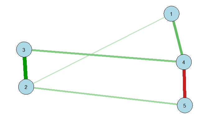
Weighted Undirected Network Graph

Consider a weighted but undirected network with five nodes, $v_1$ to $v_5$. The adjacency matrix A is represented as:

In this matrix:

• The element $A_{12} = 0.2$ indicates a positive association with a weight of 0.2 between nodes $v_1$ and $v_2$.
• $A_{45} = -0.7$ signifies a negative association between nodes $v_4$ and $v_5$.
• The symmetry of the matrix suggests that the network is undirected.

In R, one might visualize this matrix with the qgraph package::

library(qgraph)
# Define an adjacency matrix
      adj <- matrix(c(
        0,   0.2, 0,   0.5, 0,
        0.2, 0,   0.8, 0,   0.3,
        0,   0.8, 0,   0.4, 0,
        0.5, 0,   0.4, 0,   -0.7,
        0,   0.3, 0,   -0.7, 0
      ), nrow = 5, byrow = TRUE)
# Plot the graph
qgraph(adj, layout = "spring", labels = 1:5, color = "lightblue")

Unweighted Directed Network

Now consider a unweighted but directed network with five nodes, $v_1$ to $v_5$. Unlike undirected networks where relationships are mutual, directed networks allow for one-way connections, meaning node i can influence node j without node j necessarily influencing node i.

The adjacency matrix A for an unweighted directed network can be represented as:

In this matrix:

• $A_{ij} = 1$: Indicates a directed edge from node i to node j.
• $A_{ij} = 0$: Indicates no directed edge from node i to node j.
• Asymmetry: The matrix is asymmetric because $A_{ij} \neq A_{ji}$ in many cases, reflecting the one-way nature of connections in directed networks.

A quick visualization in R could be done as follows:

A <- matrix(c(
  0, 1, 0, 1, 0,
  0, 0, 1, 0, 1,
  1, 0, 0, 1, 0,
  0, 1, 0, 0, 1,
  1, 0, 1, 0, 0
  ), nrow = 5, byrow = TRUE)
      
# Plot the directed graph
qgraph(A, layout = "circle", labels = 1:5, color = "lightblue", 
          directed = TRUE, arrows = TRUE)

The difference in qgraph is we need to tell the argument that directed = TRUE, arrows = TRUE. The resulting plot would show directed arrows indicating the direction of influence.

Example: A correlation network between persons

In previous sections, we discussed fundamental concepts of network analysis in psychology, highlighting how variables (e.g., symptoms or cognitive processes) can be represented as nodes, and how their interrelationships can be depicted as edges. We now turn to a hands-on example showing how to construct a correlation network from cross-sectional data and refine it using partial correlations and model selection techniques.

First step: Correlation Networks in Cross-Sectional Analysis

In psychological research, unlike sociology, “relational data” (e.g., direct interactions among individuals) are rarely collected. Instead, cross-sectional datasets are commonly used, where each participant contributes data on a set of psychological variables at a single point in time. To build a correlation network from these data, we typically follow these steps:

1. Data Collection: Gather data from a sample of individuals on various psychological measures (e.g., symptom subdimensions, trait).
2. Correlation Matrix Computation: Calculate the correlation matrix from the person-variable data matrix. This matrix reflects the pairwise correlations between all variables (e.g., symptoms) across the sample.
3. Network Estimation: Use the correlation matrix as an adjacency matrix, treating each variable as a node and each correlation as an edge linking two nodes.

Considering the study we just introduced, We want to build a correlation network among these 11 subdimensions. Before constructing the correlation matrix, we must deal with missing data.

Before that, we should rule out any missing values. According to the original study, the approach involves removing entire participants (subjects) who have any missing values in the dataset, not just missing values within the 11 symptom subdimensions. This means that if a participant has an NA in any variable—whether it’s related to symptoms, demographic data, or other psychological measures—they are excluded from the analysis.

This is a tricky step because the presence of missing data can significantly distort the network structure, particularly when correlations are computed. To highlight the impact of this decision, it’s recommended to compare two approaches:

1. Excluding participants with any NA values across all variables (as per the original study).
2. Excluding participants only when they have NA values within the 11 symptom subdimensions.

Therefore, we followed here the original study’s rigorous exclusion criteria to ensure the network results are more comparable to their findings.

set.seed(123) # set seed to ensure the results reproducible

eat_clean <- na.omit(eat) # Excluding participants with any NA values across all variables

ed <- eat_clean[, 1:11] # choose the variables about 11 symptom subdimensions

The bootnet package in R is a powerful tool for estimating of psychological networks. It offers functionalities to estimate network structures and assess their robustness through bootstrapping methods. For a comprehensive tutorial on using the bootnet package, refer to Epskamp et al. (2018).

library(bootnet) # Load the 'bootnet' package for network estimation

cor_ed <- estimateNetwork(ed, default = 'cor') # correlation network

## Estimating Network. Using package::function:
##   - psych::corr.p for significance thresholding

plot(cor_ed) # Plot the estimated correlation network

save_layout <- plot(cor_ed)$layout # save the layout

Considerations in Network Visualization: When visualizing networks, Layout algorithms often optimize node placement based on the network’s structure, which can shift nodes between plots. Saving and reusing the layout preserves node positions across different analyses—making it easier to see how the network changes when you alter methods (e.g., partial correlation vs. correlation) or apply model selection.

Second step: Partial correlations network

While correlation networks are useful, they do not distinguish between direct relationships (edges representing direct influence) and indirect relationships (edges driven by mutual connections to other variables). For example, variable A might correlate with variable B primarily because both are correlated with variable C.

Partial correlation networks address this limitation by estimating each pairwise relationship while controlling for the influence of all other variables in the set. This approach often yields a clearer picture of direct connections among variables. A nonzero edge in a partial correlation network suggests a direct association between two variables, once all other variables are held constant.

Again, we use estimateNetwork() from the bootnet package, but set default = ‘pcor’ to compute partial correlations:

pcor_ed <- estimateNetwork(ed, default = 'pcor') # partial correlation network

## Estimating Network. Using package::function:
##   - qgraph::qgraph(..., graph = 'pcor') for network computation
##   - psych::corr.p for significance thresholding

plot(pcor_ed, layout = save_layout) # used the saved layout 

This typically produces a sparser network than the correlation network and gives more interpretable information about which variables directly influence one another.

Third step: Model selection

Even with partial correlation networks, you might end up with a fully connected or nearly saturated graph if your sample size is large enough. Such dense networks can be difficult to interpret and may include many edges of trivial or questionable significance. To address this, model selection techniques are employed to simplify the network by removing less important edges, adhering to the principle of Occam’s Razor, which advocates for the simplest model that adequately explains the data.

To go deeper of the techniques of model selection, we first explained two concepts: Independence Model: An independence model is a simple model that assumes all variables are mutually independent, implying no relationships (edges) between nodes in the network. In this model, the absence of edges suggests that knowing the state of one variable provides no information about the state of another. While this model is highly parsimonious, it is often unrealistic in psychological research, where variables are typically interrelated.

Saturated Model: In contrast, a saturated model is a highly complex model that includes a parameter for every possible relationship between variables, resulting in a fully connected network. This model perfectly fits the observed data because it accounts for all variances and covariances among variables. However, such a model can lead to overfitting, capturing noise rather than underlying patterns, and may lack interpretability due to its complexity.

Model selection aims to find a middle ground, removing weaker or non-significant edges to yield a more tractable network. Two widely used methods in psychological network analysis are pruning and regularization.

Pruning

Pruning removes edges from a saturated network based on specific criteria (e.g., significance testing or minimum effect-size thresholds).

The process of pruning involved:

1. Start with a fully connected model (every variable is linked to every other).

2. Apply criteria such as statistical significance or a minimum threshold (e.g., correlation > 0.1).

3. Remove edges that do not meet the criterion.

The advantage of Pruning is:

Computational Speed: Pruning is relatively straightforward and fast.

Unbiased Estimates: Unlike regularization methods that shrink edge weights and can introduce bias, pruning retains edges without altering their estimated strengths. Therefore, the parameter estimates for the remaining edges are unbiased.

The disadvantage of Pruning is: Potential Over-Simplification: By removing edges solely based on significance thresholds, pruning may exclude weaker but meaningful connections, especially in complex psychological networks with small effect sizes.

Risk of False Positives: Multiple significance tests can result in some edges being incorrectly retained.

Instability in Small Samples: Pruning decisions can vary substantially with different samples, reducing replicability.

pcor_ed_sig <- estimateNetwork(ed, default = "pcor", threshold = "sig") # Keep only statistically significant correlations

## Estimating Network. Using package::function:
##   - qgraph::qgraph(..., graph = 'pcor') for network computation
##   - psych::corr.p for significance thresholding

plot(pcor_ed_sig, layout = save_layout) # used the saved layout 

While pruning offers a straightforward approach to model selection by simplifying networks, it is essential to consider its limitations. Alternative methods, such as regularization techniques, may provide more robust solutions by systematically penalizing less significant edges, leading to more stable and interpretable network models.

Regularization

Regularization is a more sophisticated technique borrowed from machine learning. It systematically shrinks edge weights toward zero based on a penalty function, effectively removing weaker edges and retaining only stronger connections. The most commonly used form in psychological networks is the Graphical Lasso (particularly EBICglasso).

EBICglasso: For continuous variables, the Extended Bayesian Information Criterion Graphical Least Absolute Shrinkage and Selection Operator (EBICglasso) is a widely used method. EBICglasso balances model fit against complexity (via the Information Criterion). Small partial correlations are shrunk to zero, leading to a sparser network.

The advantages of Regularization is:

Applicability to Small Sample Sizes: By penalizing complexity, it avoids overfitting, which is especially important for datasets with many variables relative to sample size.

Improved Visual Representation: Produces a simpler, more interpretable network by eliminating minor edges.

Regularization has become a mainstream method in psychological network analysis, offering the advantage of constructing simplified and interpretable models. However, it is essential to remain mindful of its limitations:

Biased Estimates: The shrinkage of edge introduces bias into the parameter estimates, which may affect the accuracy of the inferred relationships.

Performance in Dense Networks: In situations where the true underlying network is dense, regularization may perform poorly by oversimplifying the network and omitting meaningful connections.(Empskamp et al., 2017)

pcor_ed_lasso <- estimateNetwork(ed, default = "EBICglasso") # EBICglasso Regularization

## Estimating Network. Using package::function:
##   - qgraph::EBICglasso for EBIC model selection
##     - using glasso::glasso

## Warning in EBICglassoCore(S = S, n = n, gamma = gamma, penalize.diagonal = penalize.diagonal, : A
## dense regularized network was selected (lambda < 0.1 * lambda.max). Recent work indicates a possible
## drop in specificity. Interpret the presence of the smallest edges with care. Setting threshold = TRUE
## will enforce higher specificity, at the cost of sensitivity.

plot(pcor_ed_lasso, layout = save_layout) # used the saved layout

default = “EBICglasso”: Instructs the estimateNetwork function to use the EBICglasso approach.

When estimating, you might encounter a warning. This warning indicates that the selected network is densely connected, corresponding to a low regularization parameter. In such cases, the model includes many edges, some of which may represent weak or spurious connections. Consequently, the specificity of the model—the ability to correctly identify the absence of edges—may decrease, leading to potential false positives. To mitigate concerns about specificity, you can set the threshold parameter to TRUE. This action enforces higher specificity by removing weaker edges, but it may reduce sensitivity—the ability to detect true edges.

However, this warning is not necessarily problematic. If, based on theoretical considerations or prior knowledge, you expect the true underlying network to be densely connected, a model with many edges may be appropriate. In our case, since we are analyzing 11 subdimensions of symptoms, we are not concerned about this warning because a denser network may accurately reflect the complex relationships among these symptoms within the same psychological construct.

Extra: Technical detail about EBICLASSO

The Least Absolute Shrinkage and Selection Operator (Lasso) is a statistical method used in regression analysis with machine learning to enhance both the prediction accuracy and interpretability of models.

In regression analysis, the goal is to estimate coefficients that quantify the influence of multiple predictors on an outcome variable. However, when dealing with a large number of predictors, some may contribute little to the model, potentially leading to overfitting and reduced interpretability. This challenge highlights the need for methods like Lasso, which can effectively identify and retain only the most relevant predictors while reducing the influence of less significant ones.

Lasso addresses this issue by adding a penalty term to the regression model. This penalty is proportional to the sum of the absolute values of the coefficients (known as the L1 norm). The strength of this penalty is controlled by a parameter, often denoted as λ (lambda).

The objective function for Lasso regression can be expressed as:

$\$\$\; \backslash text\{Minimize\}\; \backslash left(\; \backslash sum\; (y\_i\; -\; \backslash hat\{y\}\_i)^2\; +\; \backslash lambda\; \backslash sum\; |\backslash beta\_i|\; \backslash right)\; \$\$$

Here:

• The Sum of Squared Errors measures the difference between the observed and predicted values, known as OLS estimator in regression.
• The penalty term $\lambda \sum |\beta_i|$ imposes a constraint that encourages sparsity in the model.

The Role of Lambda (λ)

The parameter λ (lambda) plays a crucial role in Lasso regression:

• When λ = 0: The penalty term has no effect, and Lasso performs like standard linear regression, potentially including all predictors in the model.
• As λ increases: The penalty becomes more substantial, shrinking more coefficients toward zero. This leads to the exclusion of less significant predictors, resulting in a sparser model.
• If λ is too large: The model may become overly simplistic, excluding important predictors and leading to underfitting.

Selecting an appropriate value for λ is essential for balancing model complexity and predictive accuracy.

## Warning: Paket 'glasso' wurde unter R Version 4.3.1 erstellt

Understanding Bias in Coefficient Estimates

One notable limitation of Lasso is the bias introduced in the estimation of coefficients. Unlike traditional regression, where coefficients are estimated purely based on minimizing the prediction error, Lasso introduces a penalty that shrinks coefficients toward zero. This shrinkage causes the estimates of the retained coefficients to be biased because they are systematically pulled closer to zero than their true values.

• Why This Happens: The penalty term prioritizes simplicity (sparser models) over perfect accuracy in coefficient estimation. As a result, even strong predictors may have their coefficients underestimated if λ is large.
• Trade-off: While this bias reduces the variance of the model (making it more stable across different datasets), it comes at the cost of slightly distorted coefficient estimates. However, this trade-off often improves overall predictive performance, especially in high-dimensional data where overfitting is a concern.

EBIC

The EBICglasso is a method designed to achieve this balance by combining regularization techniques with model selection criteria.

Information criteria (we have learned before) are statistical tools used to compare and select models based on their fit to the data and complexity. A commonly used criterion is the Bayesian Information Criterion (BIC), which is calculated as:

$\$\$\; \backslash text\{BIC\}\; =\; -2\; \backslash times\; \backslash log(L)\; +\; k\; \backslash times\; \backslash log(n)\; \$\$$

Where:

• $L$ is the likelihood of the model,
• $k$ is the number of parameters in the model,
• $n$ is the sample size.

The Extended BIC (EBIC) extends the BIC by adding a tuning parameter $\gamma$ to control the penalty for model complexity, especially in high-dimensional settings:

$\$\$\; \backslash text\{EBIC\}\; =\; \backslash text\{BIC\}\; +\; 4\; \backslash times\; \backslash gamma\; \backslash times\; \backslash log(p)\; \$\$$

Where:

• $p$ is the total number of possible predictors or variables in the model,
• $\gamma$ is a parameter (typically between 0 and 1) that adjusts the strength of the penalty for model complexity.

A higher $\gamma$ value increases the penalty for complexity, leading to sparser models. However, the gamma is fixed to 0.5 in network analysis.

The EBICglasso Method

The EBICglasso method integrates the Graphical Lasso with the Extended BIC to select the optimal model. Here’s how it works:

1. Regularization Path: The Glasso algorithm is applied across a range of regularization parameters $\lambda$. Each $\lambda$ value results in a different network structure, with higher $\lambda$ values producing sparser networks.

2. Model Evaluation: For each network structure corresponding to a $\lambda$ value, the EBIC is calculated to assess the model’s goodness-of-fit while penalizing complexity.

3. Optimal Model Selection: The network structure with the lowest EBIC value is selected as the optimal model, achieving a balance between fit and simplicity.

By evaluating models across different $\lambda$ values, the EBICglasso method ensures that the selected network is neither too complex (overfitting) nor too simple (underfitting), providing a parsimonious representation of the relationships among variables.

Network Measures in Psychological Network Analysis

After learning how to estimate psychological networks (e.g., via correlation, partial correlation, and model selection), the next critical step is to characterize and interpret the resulting network. Network measures allow researchers to quantify the roles and relationships of individual nodes (local measures) and to assess the overall properties of the network (global measures). These metrics can help identify influential symptoms or constructs, examine how information or activation spreads throughout the network, and detect potential tipping points in mental health.

Local Measures (Nodes/Edges)

Local measures focus on the properties of individual nodes or small groups of nodes and their immediate edges.

Centrality

Centrality captures how important or influential a node is within the network. In psychopathology research, nodes with higher centrality may play a critical role in the onset or maintenance of a disorder. By intervening on these central nodes (e.g., highly connected symptoms), clinicians may disrupt the network and achieve broader therapeutic effects.

Why Centrality Matters:

• Central nodes may maintain or exacerbate disorders due to their strong connections with other symptoms.
• Intervening on central nodes could lead to cascading effects, indirectly improving related symptoms.

1. Node Strength (Degree Centrality)

Definition: The sum of the absolute weights of all edges connected to a node.

• Formula:$\$\$\; S\_i\; =\; \backslash sum\_\{j=1\}^\{n\}\; |w\_\{ij\}|\; \$\$$

  Where:

  • $S_i$ = Strength of node $i$
  • $w_{ij}$ = Weight of the edge between node $i$ and node $j$
  • $n$ = Total number of nodes

• Interpretation: A node with a high strength value has many strong connections. In a symptom network, this might be a symptom that co-occurs strongly with several others, suggesting a pivotal role in the disorder’s structure.

To compute the strength of nodes, we can apply the following code:

library(qgraph)

# Generate a centrality plot for the partial correlation network
centralityPlot(
  pcor_ed_lasso, # Partial correlation network estimated using Lasso
  include = c("Strength") # Include only 'Strength' as the centrality measure
)

2. Expected Influence (Degree Centrality)

Definition: An alternative centrality metric that retains the sign of the edges (positive or negative) rather than using absolute values.

• Formula:$\$\$\; \backslash text\{ExpectedInfluence\}$1(i) = \sum{j=1}^{n} a_{ij} w_{ij} $$

  Where:

  • $a_{ij} = 1$ if nodes $i$ and $j$ are connected, otherwise $0$
  • This measure reflects how much activating (or deactivating) a node would affect other nodes directly.

• Why It better than Strength: In psychopathology, positive edges (e.g., anxiety ↔ worry) might exacerbate each other, whereas negative edges (e.g., self-esteem ↔ depression) can have opposing dynamics. Expected Influence captures these differences directly.

The following code can be used to calculate node Expected Influence, it is nearly same as Strength but with argument include = c(“Strength”):

library(qgraph)

centralityPlot(
  pcor_ed_lasso,
  include = c("ExpectedInfluence") # Include only 'ExpectedInfluence' as the centrality measure
)

3. Closeness Centrality (Closeness Centrality)

Definition: How quickly a node can reach (or be reached by) all other nodes via the shortest paths. It’s the inverse of the sum of the shortest path distances from a node to all other nodes.

• Formula:$\$\$\; \backslash text\{Closeness\}(i)\; =\; \backslash frac\{1\}\{\backslash sum\_\{j=1\}^\{n\}\; \backslash text\{Distance\}(i,\; j)\}\; \$\$$

  Where:

  • $\text{Distance}(i, j)$ = Shortest path length between nodes $i$ and $j$
  • $n$ = Total number of nodes

• Interpretation: A node with high closeness can rapidly affect or be affected by other symptoms. In clinical contexts, such a node might accelerate the spread of distress (or recovery) across the entire symptom network.

Here’s an example of code that helps compute node closeness with argument include = c(“Closeness”):

library(qgraph)

centralityPlot(
  pcor_ed_lasso,
  include = c("Closeness") # Include only 'Closeness' as the centrality measure
)

4. Betweenness Centrality (Betweenness Centrality)

Definition: How often a node lies on the shortest path between other node pairs.

• Formula:$\$\$\; \backslash text\{Betweenness\}(i)\; =\; \backslash sum\_\{j\; \backslash neq\; k\}\; \backslash frac\{\backslash sigma\_\{jk\}(i)\}\{\backslash sigma\_\{jk\}\}\; \$\$$

  Where:

  • $\sigma_{jk}$ = Total number of shortest paths between nodes $j$ and $k$
  • $\sigma_{jk}(i)$ = Number of those paths that pass through node $i$

• Interpretation: A node with high betweenness is a “bridge” or “bottleneck” in the network. However, betweenness is often unstable in psychological research, especially with smaller samples, because minor data variations can drastically change shortest paths. Consequently, betweenness centrality is often not recommended for psychological network analysis. Closeness centrality, which assesses how close a node is to all other nodes in the network, also exhibits instability but tends to be more reliable than betweenness centrality, seeing more information in Hallquist et al., (2021).

The code provided below allows us to measure the Betweenness of nodes with argument include = c(“Betweenness”):

library(qgraph)

centralityPlot(
  pcor_ed_lasso,
  include = c("Betweenness") # Include only 'Betweenness' as the centrality measure
)

Centrality Difference Test in Psychological Networks

Researchers often want to test if the centrality scores of two nodes differ significantly (e.g., strength, closeness, betweenness). This is typically done via a non-parametric bootstrap procedure (Epskamp et al., 2018):

1. Resampling: Repeatedly draw samples from the original dataset with replacement.

2. Centrality Calculation: For each resampled dataset, compute the centrality indices (e.g., expected influence) for the nodes under investigation.

3. Difference Assessment: Calculate the difference in centrality measures between the two nodes for each resampled dataset.

4. Confidence Intervals: Generate 95% confidence intervals for the distribution of these difference scores.

5. Significance Testing: Examine whether the confidence interval includes zero:

   • If zero is not within the interval, the difference is considered statistically significant.
   • If zero falls within the interval, the difference is not statistically significant.

Visualization often uses a matrix-style plot:

• Gray Boxes: Indicate pairs of nodes whose centrality measures do not differ significantly.

• Black Boxes: Represent pairs of nodes with significantly different centrality measures.

• White Boxes: Display the centrality value of individual nodes.

It’s important to note that testing differences among all node pairs can inflate Type I error. Adjustments or cautious interpretation may be necessary.

Here’s an example using the bootnet package in R to conduct a non-parametric bootstrap procedure for testing differences in expected influence:

# Perform non-parametric bootstrap with 1000 iterations
boot_diff <- bootnet(
  pcor_ed_lasso,                # The estimated network object
  nBoots = 1000,                # Number of bootstrap samples
  default = "EBICglasso",       # Default method for network estimation
  statistics = "ExpectedInfluence",  # Centrality measure to assess
  type = 'nonparametric',        # Non-parametric bootstrap, very important
  verbose = F 
)

# Plotting the centrality difference results
plot(
  boot_diff,
  statistics = "ExpectedInfluence",  # Plot expected influence differences
  order = "sample",                 # Orders nodes based on sample centrality
  labels = TRUE                     # Displays node labels in the plot
)

Clustering of Nodes

Clustering measures how nodes group into tightly interconnected sub-networks or communities.

Analogy: Consider symptoms as viruses spreading within a population. In highly clustered groups, symptoms can rapidly “infect” each other, leading to quick propagation within the cluster.

Implication for Interventions:

1. Cluster-Level Treatment Impact: Treating a central symptom in a cluster may yield improvements in the entire cluster.

2. Differential Recovery Rates: Symptoms in separate clusters may show slower change if they are weakly connected to the treated cluster.

Global Measures (The Whole Graph Properties)

Local measures focus on individual nodes or small clusters. Global measures describe the overall structure and efficiency of the entire network, offering insight into how information or activation spreads system-wide.

1. Connectivity (Network Efficiency)

Connectivity indicates how densely nodes are connected. Highly connected (dense) networks can rapidly propagate signals, while sparsely connected networks spread signals more slowly.

Measuring Connectivity: Average Shortest Path Length (APL)

A common way to assess network efficiency is the average shortest path length (APL):

Where:

• $n$ = Total number of nodes in the network
• $d_{ij}$ = Shortest path distance between nodes $i$ and $j$

Interpretation:

• Low APL: High efficiency—information spreads quickly (common in dense networks).
• High APL: Low efficiency—information spreads slowly (common in sparse networks).

Importance in Psychopathology:

In dynamical systems theory, a network can exhibit attractor states—patterns in which the system settles, such as a stable mental health state or a chronic disorder state. Changes in connectivity(APL) can foreshadow critical transitions (tipping points) between these states.

In networks with low connectivity, nodes have fewer connections, leading to weaker interactions among symptoms. Such networks are typically more stable and less susceptible to widespread activation, corresponding to a stable mental health or a stable mental disorder.

Highly connected networks feature numerous and strong interactions among nodes. This configuration can facilitate rapid and extensive spread of activation across the network, potentially leading to a mental disorder state where symptoms reinforce each other, creating a self-sustaining pattern of activation.

Ball-and-Valley Metaphor

Deep Valley: A stable attractor. Small pushes (stressors) do not move the system out of the valley.

Shallow Valley: A fragile or unstable attractor. Minor stressors can push the system over the edge into another valley (potentially a disordered state).

Increasing Connectivity: Flattens or shallows the “valley,” making it easier for the system (the ball) to roll into a new, potentially adverse attractor.

A critical transition refers to a sudden shift from one attractor state to another, often precipitated by gradual changes in system parameters, such as increasing connectivity or external stressors. As the system approaches a critical point, it may exhibit early warning signals, including increased connectivity in symptom dynamics.

Understanding these dynamics is crucial for identifying early warning signals of mental health deterioration. Monitoring changes in network connectivity and symptom activation patterns can help predict impending critical transitions, allowing for timely interventions to restore the system to a stable, healthy attractor state.

2. Small-Worldness

Small-world networks are characterized by:

• High Clustering Coefficient among nodes .
• Short path lengths: overall.

The Global Clustering Coefficient (C) measures the extent to which nodes in a network cluster together, forming tightly connected groups.

Where:

• $C_i = \frac{\text{Number of triangles connected to node } i}{\text{Number of triplets centered at node } i}$
• Triangles: Groups of three nodes where each node is connected to the other two.
• Triplets: Sets of three nodes where at least two are connected.

Interpretation:

• High C and Low APL = A robust small-world network that can transmit information efficiently while maintaining local specialization.

• Low C or High APL = Less efficient network with weaker clustering.

Famous Examples:

• Six Degrees of Separation: Suggests that any two people on Earth are connected by no more than six acquaintances.
• Social Networks: The concept of “The Strength of Weak Ties” highlights the role of weak connections in bridging different social groups.

Significance in Clinical Psychology and Psychiatry:

The human brain’s architecture exemplifies small-world network properties, effectively balancing local specialization and global integration. This configuration enables efficient information processing, which is essential for both cognitive and emotional functions. In a small-world network, nodes (representing neurons or brain regions) are highly clustered, facilitating specialized processing within local groups. Simultaneously, short path lengths between clusters allow for rapid communication across the entire network, ensuring cohesive integration of information. This dual organization supports the brain’s ability to perform complex tasks by maintaining a balance between segregated (specialized) and integrated (holistic) processing.

Research indicates that individuals with certain psychiatric conditions, such as schizophrenia, exhibit disruptions in these small-world network properties. Studies have found that while the brain functional networks of healthy individuals display efficient small-world characteristics, these properties are altered in patients with schizophrenia. For example, a dysfunctional integration within the brain’s network in schizophrenia, potentially contributing to the cognitive and emotional challenges (such as hallucination) associated with the disorder.

To calculate all global network measures, we can use the smallworldIndex() function from the qgraph package in R. This function computes important metrics such as clustering coefficient, average shortest path length (APL), and the small-world index, which help to assess the efficiency and structural properties of the network.

Here’s the R code to perform this calculation:

library(qgraph)

# Calculate global network measures
smallworldIndex(qgraph(pcor_ed_lasso$graph))

## Warning in smallworldIndex(qgraph(pcor_ed_lasso$graph)): Edge weights removed

## $transitivity
## [1] 0.9247059
## 
## $transitivity_random
## [1] 0.8429752
## 
## $APL
## [1] 1.072727
## 
## $APL_random
## [1] 1.31752
## 
## $index
## [1] 1.347276

You might encounter the following warning: Edge weights removed. This warning indicates that edge weights (the strength of connections between nodes) have been removed during the calculation of global measures. This is because many global metrics, such as the small-world index, rely solely on the presence or absence of connections (i.e., the network structure), rather than the precise strength of those connections. This approach focuses on whether nodes are connected, not how strongly they are connected. The warning simply serves as a notification that the metrics are being calculated based on an unweighted (binary) version of the network, which is the appropriate method for these types of analyses.

Stability in Network Estimations

When constructing psychological networks, it is essential to evaluate the stability of the estimated network parameters—such as edge weights and centrality measures. Stability refers to how consistently these parameters remain when the data varies (e.g., when the sample changes slightly). Because many psychological studies involve limited sample sizes, results can be sensitive to sampling variability. This section explores the importance of stability, the limitations of traditional bootstrapping, and a recommended approach known as case-dropping bootstrap for assessing centrality stability.

The Problem of Limited Sample Size

Sampling Variation: Small sample sizes lead to high sampling variation; estimates of network structure (e.g., correlation or partial correlation networks) may differ substantially if you draw a different set of participants from the same population.

Unstable Parameter Estimates: Network models rely on statistical associations. With insufficient data, parameter estimates — like edge weights and centrality indices — can fluctuate due to random noise, making conclusions less reliable.

Key Question:
How stable are the estimated parameters (e.g., edge weights, centrality measures) when the dataset changes slightly? A methodologically sound analysis must address this question to avoid overinterpreting what may be unstable results.

The Problem with Non-Parametric Bootstrap

The non-parametric bootstrap is a resampling technique where multiple new datasets are created by randomly sampling (with replacement) from the original dataset. The parameter estimates fluctuate around the true value due to natural sampling variability. Some bootstrapped samples may slightly overestimate, and others may slightly underestimate the parameter. This variability creates a distribution of estimates that centers around the true value. In order words, this distribution captures the variability from dataset, the inverse of stability.

It is used to generate Bootstrapped Confidence Intervals (BCIs) around estimated parameters to describe this distribution, aiming to capture the uncertainty of the estimates. It is what we used in the centrality difference test.

Why Does It Fail in Network Estimation?

Model Selection Bias: Regularization techniques like LASSO often set small edge weights to exactly zero during model selection. In bootstrapped samples, this can cause the same edges to repeatedly drop to zero, even if the true edge is non-zero. In the context of bootstrapping, this bias is known as model selection bias.

Consider a scenario where the true edge weight between nodes A and B in a network is 0.25. With a very small sample size (e.g., N = 10), the following occurs:

In small datasets, random sampling variability is high. This means that the observed correlations (or partial correlations) between nodes A and B can fluctuate largely across bootstrapped samples. The most of time, these fluctuations may even show a weaker correlation or no correlation at all, even though a true connection exists in the population. (the small sample is easy to have extreme results) LASSO penalizes small coefficients more aggressively. When the bootstrapped sample happens to produce a weak observed correlation (due to sampling variability), the regularization process pushes that weak edge all the way to zero. As a result, in most bootstrapped samples, the estimated edge weight between A and B will be set to zero—not because the connection doesn’t exist, but because regularization overpowers the weak signal due to sample noise. Final result: The bootstrapped confidence interval is [0, 0], erroneously excluding the true value of 0.25. Consequently, the BCIs fail to capture the true edge weight of 0.25.

Hence, non-parametric bootstrapping for regularized networks can yield biased results and underestimate the presence of real connections.

A Better Approach: Case-Dropping Bootstrap (Stability Estimates)

To address the limitations of traditional bootstrapping—particularly for centrality measures—researchers often employ the case-dropping bootstrap (also called subset bootstrap). This method assesses how robust centrality estimates are when subsets of the data are systematically removed.

How It Works:

1. Full Dataset Analysis:Compute centrality measures (e.g., node strength, expected influence) using all participants.
2. Subset Resampling: Randomly drop a certain percentage of participants (e.g., 10%) to form a new subset.
3. Recompute Centrality: Calculate centrality measures for the subset.
4. Repeat: Perform this process for increasing proportions of dropped cases (10%, 20%, 30%, …, up to 90%).
5. Correlation Stability Coefficient (CS-Coefficient): For each dropout proportion, compute how well the subset-based centrality measures correlate with the original (full-data) centrality. Summarize these correlations as a function of dropout proportion.

Below is an example using the bootnet package. We assume you have already estimated a network object (e.g., pcor_ed_lasso) using EBICglasso:

# Perform case-dropping bootstrap to assess stability of expected influence
stab_diff <- bootnet(
  pcor_ed_lasso,       # estimated network
  nBoots = 1000,       # Number of bootstrap samples
  default = "EBICglasso", # Network estimation method
  type = 'case',       # Case-dropping bootstrap, very important
  statistics = c("expectedInfluence"), # Centrality measure to assess
  verbose = F
)


# Calculate the correlation stability coefficient
corStability(stab_diff, cor = 0.7)

## === Correlation Stability Analysis === 
## 
## Sampling levels tested:
##    nPerson Drop%   n
## 1      249  75.0  93
## 2      326  67.3  93
## 3      404  59.4 107
## 4      481  51.7 109
## 5      559  43.9  87
## 6      636  36.1 112
## 7      714  28.3 103
## 8      791  20.6  98
## 9      869  12.8 104
## 10     946   5.0  94
## 
## Maximum drop proportions to retain correlation of 0.7 in at least 95% of the samples:
## 
## expectedInfluence: 0.75 (CS-coefficient is highest level tested)
##   - For more accuracy, run bootnet(..., caseMin = 0.673, caseMax = 1) 
## 
## Accuracy can also be increased by increasing both 'nBoots' and 'caseN'.

This analysis involves creating multiple bootstrap samples by systematically removing increasing proportions of the original dataset (from 5% up to 75%). For each specified drop percentage, a set number of bootstrap samples (denoted by ’n’) is generated. For instance, when 75% of the data is removed, 99 bootstrap samples are created, each containing 25% of the original participants (249 out of the initial total).

For the “expected influence” statistic, the CS coefficient is reported as 0.75. This indicates that up to 75% of the sample can be removed, and the correlation between the original and subsetted centrality measures will remain at or above 0.7 traditional correlation in at least 95% of the bootstrap samples. However, the aimed correaltion could be changed, for example, cor = 0.8 to change to 0.8 traditional correlation.

The result suggests that the stability is robust, as 0.75 was the maximum proportion tested. To determine the exact maximum drop proportion (but usually do not needed), the function recommends adjusting the caseMin and caseMax parameters in the bootnet function to test higher proportions.

Interpreting the CS-Coefficient:

• CS ≥ 0.5 (preferable): Indicates strong stability. The centrality estimates are reliable even when up to 50% of the data is removed.
• CS between 0.25 and 0.5: Moderate stability. The estimates may still be acceptable but should be interpreted cautiously.
• CS < 0.25: Poor stability. The centrality measures are likely unreliable.

It’s important to note that the CS-Coefficient is distinct from the traditional correlation coefficient. CS-Coefficient Evaluates the stability of centrality indices in a network by determining how much of the data can be removed while still maintaining a high correlation between the original and subsetted centrality measures. Represents the maximum proportion of the sample that can be dropped while retaining, with a 95% confidence interval, a traditional correlation of at least 0.7 between the centrality measures of the original and subsetted data.

Example Visualization:

plot(stab_diff, "expectedInfluence")

• The plot shows the average correlation between the original centrality estimates and those obtained after progressively dropping participants.
• As more data is removed, the correlation typically decreases, but stable networks maintain relatively high correlations even with substantial case-dropping.

In this plot:

• A high correlation (closer to 1.0, here is traditional correlation) indicates that the centrality estimates are stable.
• A sharp drop-off in correlation as more cases are removed suggests instability.

Advanced Topics in Psychological Network Analysis

As psychological network analysis evolves, several advanced techniques have emerged to provide deeper insights into the structure and dynamics of psychological constructs. This section introduces four usually used advanced topics:

1. Exploratory Graph Analysis (EGA)

Exploratory Graph Analysis (EGA) is a data-driven method designed to uncover latent structures within psychological networks. It identifies communities (also referred to as clusters, we have leared in the local measures) of variables (nodes), which are conceptually similar to factors in traditional latent variable models like factor analysis.

Key Concepts:

• Communities in Networks ≈ Clusters of Variables (Nodes) ≈ Factors in latent variable models (e.g., personality traits).
• Purpose: Identify groups of closely related nodes that may represent underlying psychological constructs (e.g., dimensions of depression or anxiety).

How It Works:

• Community Detection Algorithms: EGA applies algorithms such as the Walktrap Algorithm or Louvain Method to detect clusters of related nodes based on their connectivity patterns.
• Dimensionality Exploration: Helps in determining the number and nature of latent dimensions underlying psychological data, offering an alternative to traditional exploratory factor analysis (EFA).

Applications:

• Identifying dimensions of mental disorders (e.g., subtypes of depression).
• Understanding personality structure beyond conventional factor models.

For a comprehensive understanding of EGA, consider reading Golino and Epskamp’s (2017) article, “Exploratory graph analysis: A new approach for estimating the number of dimensions in psychological research.”

2. Bridge Centrality

Bridge Centrality measures the role of a node as a “bridge” between different communities within a network. Nodes with high bridge centrality facilitate communication or activation spread between otherwise distinct clusters.

Why It Matters:

• In psychopathology, bridge nodes can explain comorbidity between disorders. For example, a symptom like “sleep disturbances” might connect clusters representing depression and anxiety, contributing to their co-occurrence.

Bridge Expected Influence Formula:

Where:

• $N(i)$ = The set of neighbors directly connected to node $i$.
• $C$ = Nodes in a community different from that of node $i$.
• $w_{ij}$ = The weight of the edge between nodes $i$ and $j$.

Interpretation:

• Higher Bridge Centrality: Indicates a node’s strong influence across different communities.
• Clinical Implication: Targeting bridge symptoms in treatment may reduce comorbidity and improve outcomes.

For more detailed information on bridge centrality, refer to Jones et al.’s (2021) study on its application in psychopathology.

3. Network Comparison Between Groups

Network Comparison allows researchers to assess whether network structures differ between groups, such as clinical vs. control populations.

Key Objectives:

• Compare edge weights (strength of relationships).
• Assess differences in centrality measures (importance of nodes).
• Identify unique sub-network patterns across groups.

Methods: Network Comparison Test (NCT)

The Network Comparison Test (NCT) is a permutation-based method used to statistically assess differences between two networks. This approach evaluates whether observed disparities in network structures are significant or could have arisen by chance.

Detailed Procedure:

1. Combine Data:

   • Merge the datasets from the two groups under comparison into a single pooled dataset.

2. Calculate Observed Test Statistic:

   • Compute the network for each group separately.
   • Determine the test statistic of interest (e.g., global strength difference, specific edge weight differences) between the two networks.

3. Permutation Process:

   • Shuffle Group Labels:
     • Randomly reassign the group labels of the pooled dataset to create two new groups.
   • Recompute Networks:
     • Construct networks for these newly formed groups using the same estimation methods as applied to the original data.
   • Calculate Test Statistic:
     • Compute the test statistic for the permuted groups.
   • Repeat:
     • Perform the shuffling and computation multiple times (typically 1,000 or more) to build a distribution of the test statistic under the null hypothesis that there is no difference between the groups.

4. Assess Significance:

   • Compare the observed test statistic to the distribution of permuted test statistics.
   • The p-value is determined by the proportion of permuted test statistics that are as extreme as or more extreme than the observed test statistic.

The NCT provides a robust framework for comparing network structures between groups. By leveraging permutation methods, it assesses the likelihood that observed differences are due to chance, thereby offering insights into the distinctiveness of network characteristics across populations.

Example:

• Comparing the symptom network of individuals with major depressive disorder (MDD) to that of healthy controls to identify key differences in symptom connectivity.

For a deeper dive into network comparison methods, see Van Borkulo et al.’s (2023) work on the Network Comparison Test.

4. Confirmatory Network Modeling (CNM)

While exploratory methods like EGA identify latent structures without prior hypotheses, Confirmatory Network Modeling (CNM) is a hypothesis-driven approach that tests specific, pre-defined network structures.

How It Works:

• Combines principles from Confirmatory Factor Analysis (CFA) with network modeling techniques.
• Researchers specify expected relationships (edges) between variables based on theoretical models.

Applications:

• Testing theoretical models of psychological constructs (e.g., validating the cognitive-behavioral model of depression).
• Replicating or confirming hypothesized relationships in different datasets.

Benefits:

• Enables formal statistical testing of network structures.
• Useful for validating intervention targets based on theoretical frameworks.

For more on CNM, consider reading Isvoranu et al.’s (2022) discussion on confirmatory network analysis.

Summary

These four advanced network analysis techniques enhance the ability to explore, compare, and confirm psychological models:

By integrating these methods, researchers can move beyond simple descriptive models to a deeper understanding of the complex dynamics underlying psychological phenomena.

References

Cohen, J. (1988). Statistical power analysis for the Behavioral Sciences. Routledge.

Cramer, A. O., Waldorp, L. J., Van Der Maas, H. L., & Borsboom, D. (2010). Comorbidity: A network perspective. Behavioral and brain sciences, 33(2-3), 137–150.

Epskamp, S., Kruis, J., & Marsman, M. (2017). Estimating psychopathological networks: Be careful what you wish for. PloS one, 12(6), e0179891.

Golino, H. F., & Epskamp, S. (2017). Exploratory graph analysis: A new approach for estimating the number of dimensions in psychological research. PloS one, 12(6), e0174035.

Gordon, R. P., Brandish, E. K., & Baldwin, D. S. (2016). Anxiety disorders, post-traumatic stress disorder, and obsessive–compulsive disorder. Medicine, 44(11), 664–671.

Hallquist, M. N., Wright, A. G., & Molenaar, P. C. (2021). Problems with centrality measures in psychopathology symptom networks: Why network psychometrics cannot escape psychometric theory. Multivariate behavioral research, 56(2), 199-223.

Isvoranu, A.-M., Epskamp, S., Waldorp, L., & Borsboom, D. (2022). Network psychometrics with r: A guide for behavioral and social scientists. Taylor & Francis.

Jones, P. J., Ma, R., & McNally, R. J. (2021). Bridge centrality: A network approach to understanding comorbidity. Multivariate behavioral research, 56(2), 353–367.

Lange, J., Dalege, J., Borsboom, D., van Kleef, G. A., & Fischer, A. H. (2020). Toward an integrative psychometric model of emotions. Perspectives on Psychological Science, 15(2), 444–468.

Reale, L., Bartoli, B., Cartabia, M., Zanetti, M., Costantino, M. A., Canevini, M. P., Termine, C., & Bonati, M. (2017). Comorbidity prevalence and treatment outcome in children and adolescents with adhd. European child & adolescent psychiatry, 26, 1443–1457.

Van Borkulo, C. D., van Bork, R., Boschloo, L., Kossakowski, J. J., Tio, P., Schoevers, R. A., Borsboom, D., & Waldorp, L. J. (2023). Comparing network structures on three aspects: A permutation test. Psychological methods, 28(6), 1273.

Van Der Maas, H. L., Dolan, C. V., Grasman, R. P., Wicherts, J. M., Huizenga, H. M., & Raijmakers, M. E. (2006). A dynamical model of general intelligence: The positive manifold of intelligence by mutualism. Psychological review, 113(4), 842.

Vervaet, M., Puttevils, L., Hoekstra, R. H., Fried, E., & Vanderhasselt, M. A. (2021). Transdiagnostic vulnerability factors in eating disorders: A network analysis. European eating disorders review, 29(1), 86-100.