](/media/header/rainbow_loops_road.jpg)
Abschnitte:
Vorbereitung
Kontinuierliche vs. diskrete Zeit
- Kontinuierliche Zeit
- Zeit wird in “natürlichen” Einheiten (Millisekunden, Stunden, Tage, …) abgebildet
- Veränderung ist eine (stetige) Funktion der Zeit
- Eine funktionale Form wird vorgegeben (linear, quadratisch, logarithmisch)
- Aus der Funktion wird auf alle zeitlichen Abstände generalisiert
- Abstände zwischen Messungen können intra- und interindividuell variieren
- Diskrete Zeit
- Zeit wird in künstlichen Einheiten (meist Messzeitpunkten) angegeben
- Veränderung findet in Intervallen statt
- Die Form der Veränderung ist unbekannt
- Abstände zwischen Messungen müssen interindividuell identisch sein
Datenbeispiel
load(url('https://pandar.netlify.app/daten/Sunday.rda'))
head(sunday)
##   id mzp  pos  neg   gs  wm meq ctime gs_lag wm_lag
## 1  1   0 nein nein 2.00 1.0  33  2.23     NA     NA
## 2  1   1 nein nein 2.75 1.5  33  3.64   2.00    1.0
## 3  1   2   ja nein 2.00 2.5  33  5.21   2.75    1.5
## 4  1   3 nein nein 3.00 2.5  33  7.20   2.00    2.5
## 5  1   4 nein nein 3.00 2.0  33  9.57   3.00    2.5
## 6  1   5 nein nein 2.75 1.0  33 11.12   3.00    2.0
Crayen, C., Eid, M., Lischetzke, T., Courvoisier, D. S. und Vermunt, J. K. (2012). Exploring dynamics in mood regulation—Mixture latent Markov modeling of ambulatory assessment data. Psychosomatic Medicine, 74, 366-376.
- Ambulatory-Assessment Studie zur Stimmungsregulation
- Messzeitpunkte in 150 Personen (Variable id)
- Bis zu 8 Messungen pro Tag, Zeitabstand zwischen 60 und 180 Minuten
- Hier: Ein Tag (Sonntag) ausgewählt
- Berichten von Daily hassles (neg) oder Uplifts (pos)
- Momentante gute Stimmung (gs) und Wachheit (wm), erfasst mit 4 bzw. 2 vierstufigen Items
- Einmalige Einschätzung der eigenen Morningness (meq)
- Zählung der individuellen Messzeitpunkte beginnt bei 0 (mzp)
- Uhrzeit in (anteiligen) Stunden ab 8 Uhr morgens (ctime)
- Vorherige gute Stimmung (gs_lag) und Wachheit (wm_lag), erfasst mit 4 bzw. 2 vierstufigen Items
Pakete
# Für Plots der Modelle - dauert einen Moment
install.packages('sjPlot', dependencies = TRUE)

# Für eine erweiterte Modellzusammenfassung
installpackages('jtools')
Für alternative Ansätze der Darstellung bzw. Berechnung von Komponenten (nur in vereinzelten Beispielen genutzt)
# Für Inferenz der fixed effects
install.packages('lmerTest')

# Für Bestimmung von Pseudo R^2
install.packages('MuMIn')
library(lme4)
library(sjPlot)
library(jtools)
library(ggplot2)
State-Trait-Modell
Level 1 $$ y_{ti} = \beta_{0i} + r_{ti} $$
Level 2 $$ \beta_{0i} = \gamma_{00} + u_{0i} $$
Gesamtgleichung $$ y_{ti} = \gamma_{00} + u_{0i} + r_{ti} $$
- Klassisches Nullmodell, nur $t$ für “Time” und $i$ für “individual”
- Zerlegung in LST:
- $\tau_{ti}$: True Score der Person $i$ zum Zeitpunkt $t$
- $\xi_{i}$: Trait der Person $i$
- $\zeta_{ti}$: State-Abweichung vom Trait zum Zeitpunkt $t$ für Person $i$
$$ \tau_{ti} = \xi_{i} + \zeta_{ti} $$
mod0 <- lmer(wm ~ 1 + (1 | id), sunday)
print(summ(mod0))
## MODEL INFO:
## Observations: 1069
## Dependent Variable: wm
## Type: Mixed effects linear regression
##
## MODEL FIT:
## AIC = 2417.01, BIC = 2431.93
## Pseudo-R² (fixed effects) = 0.00
## Pseudo-R² (total) = 0.22
##
## FIXED EFFECTS:
## --------------------------------------------------------
##                     Est.   S.E.   t val.     d.f.      p
## ----------------- ------ ------ -------- -------- ------
## (Intercept)         2.66   0.04    71.55   152.45   0.00
## --------------------------------------------------------
##
## p values calculated using Satterthwaite d.f.
##
## RANDOM EFFECTS:
## ------------------------------------
##   Group      Parameter    Std. Dev.
## ---------- ------------- -----------
##     id      (Intercept)     0.37
##  Residual                   0.69
## ------------------------------------
##
## Grouping variables:
## -------------------------
##  Group   # groups   ICC
## ------- ---------- ------
##   id       148      0.22
## -------------------------
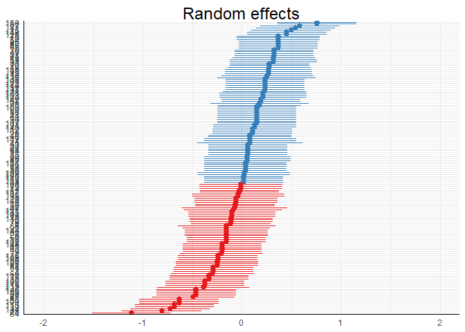
ICC: Stabilitätsausmaß (relativer Varianzanteil der Personeneigenschaften)
# Individuelle Traits (Ewartungswerte, beta0i)
coef(mod0)$id |> head()
##   (Intercept)
## 1    2.025617
## 2    2.548404
## 3    2.461273
## 4    2.374142
## 5    3.027625
## 6    2.743919
# Abweichungen (u0i)
ranef(mod0)$id |> head()
##   (Intercept)
## 1 -0.63415702
## 2 -0.11137054
## 3 -0.19850162
## 4 -0.28563270
## 5  0.36785040
## 6  0.08414454
plot_model(mod0, 're', sort.est = '(Intercept)')
Einfache Wachstumskurven
Lineares Wachstum
- Random Intercept Modell mit Zeit als UV
mod1 <- lmer(wm ~ 1 + ctime + (1 | id), sunday)
print(summ(mod1))
## MODEL INFO:
## Observations: 1069
## Dependent Variable: wm
## Type: Mixed effects linear regression
##
## MODEL FIT:
## AIC = 2418.90, BIC = 2438.80
## Pseudo-R² (fixed effects) = 0.01
## Pseudo-R² (total) = 0.23
##
## FIXED EFFECTS:
## --------------------------------------------------------
##                     Est.   S.E.   t val.     d.f.      p
## ----------------- ------ ------ -------- -------- ------
## (Intercept)         2.53   0.06    44.08   628.34   0.00
## ctime               0.02   0.01     2.96   952.29   0.00
## --------------------------------------------------------
##
## p values calculated using Satterthwaite d.f.
##
## RANDOM EFFECTS:
## ------------------------------------
##   Group      Parameter    Std. Dev.
## ---------- ------------- -----------
##     id      (Intercept)     0.37
##  Residual                   0.69
## ------------------------------------
##
## Grouping variables:
## -------------------------
##  Group   # groups   ICC
## ------- ---------- ------
##   id       148      0.23
## -------------------------
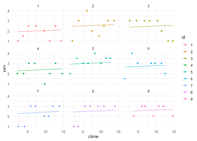
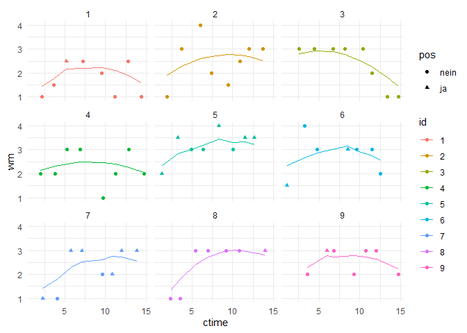
sunday$pred_mod1 <- predict(mod1)

subset(sunday, as.numeric(id) < 10) |>
  ggplot(aes(x = ctime, y = wm, color = id)) +
    geom_point() +
    geom_line(aes(y = pred_mod1)) +
    theme_minimal() + facet_wrap(~ id)
Kurvilineares Wachstum
plot_model(mod1, 'slope')
## `geom_smooth()` using formula = 'y ~ x'
## `geom_smooth()` using formula = 'y ~ x'
sunday$ct_quad <- sunday$ctime^2
cor(sunday$ctime, sunday$ctime^2)
## [1] 0.9762517
poly(sunday$ctime, 2)
##                     1             2
##    [1,] -0.0452148114  0.0374195556
##    [2,] -0.0342732643  0.0063543766
##    [3,] -0.0220901233 -0.0179246810
##    [4,] -0.0066477980 -0.0330853404
##    [5,]  0.0117433131 -0.0283674805
##    [6,]  0.0237712549 -0.0118909579
##    [7,]  0.0365751929  0.0172852502
##    [8,]  0.0493015314  0.0581760897
##    [9,] -0.0476203998  0.0454246173
##   [10,] -0.0334972681  0.0044839639
##   [11,] -0.0154165555 -0.0266182907
##   [12,] -0.0048630066 -0.0337122572
##   [13,]  0.0109673168 -0.0290668356
##   [14,]  0.0219088639 -0.0151350730
##   [15,]  0.0308328207  0.0027160449
##   [16,]  0.0441023565  0.0400383598
##   [17,] -0.0428092230  0.0298380868
##   [18,] -0.0280652944 -0.0073747309
##   [19,] -0.0106053788 -0.0308634622
##   [20,]  0.0008793656 -0.0341473218
##   [21,]  0.0183392812 -0.0206432990
##   [22,]  0.0267976402 -0.0060777683
##   [23,]  0.0413087700  0.0311099265
##   [24,]  0.0516295201  0.0669388012
##   [25,] -0.0466116046  0.0420160843
##   [26,] -0.0331868696  0.0037481408
##   [27,] -0.0216245255 -0.0186370000
##   [28,] -0.0088205875 -0.0320074180
##   [29,]  0.0131401063 -0.0269975639
##   [30,]  0.0246248508 -0.0103192210
##   [31,]  0.0370407907  0.0185723251
##   [32,]  0.0517071197  0.0672377238
##   [33,] -0.0522763772  0.0621216242
##   [34,] -0.0371444504  0.0136581646
##   [35,] -0.0241077135 -0.0146545996
##   [36,] -0.0129333676 -0.0290209230
##   [37,]  0.0020433600 -0.0339412876
##   [38,]  0.0154680951 -0.0243970055
##   [39,]  0.0268752399 -0.0059198965
##   [40,]  0.0358767963  0.0153843906
##   [41,] -0.0540611686  0.0689428713
##   [42,] -0.0374548489  0.0144839076
##   [43,] -0.0258149052 -0.0116548740
##   [44,]  0.0039057510 -0.0334053463
##   [45,]  0.0125193093 -0.0276240470
##   [46,]  0.0266424410 -0.0063921896
##   [47,]  0.0347904016  0.0124984642
##   [48,] -0.0445164148  0.0351748464
##   [49,] -0.0309364805 -0.0013756619
##   [50,] -0.0178221439 -0.0238603156
##   [51,] -0.0071133957 -0.0328834488
##   [52,]  0.0122089108 -0.0279267098
##   [53,]  0.0215984654 -0.0156510750
##   [54,]  0.0304448226  0.0018186939
##   [55,]  0.0449559524  0.0428804347
##   [56,] -0.0442060163  0.0341886583
##   [57,] -0.0349716609  0.0080754350
##   [58,] -0.0203053319 -0.0205690638
##   [59,] -0.0082773901 -0.0323092962
##   [60,]  0.0087169277 -0.0308457022
##   [61,]  0.0217536646 -0.0153939556
##   [62,]  0.0460423471  0.0465747581
##   [63,] -0.0348164617  0.0076898921
##   [64,] -0.0159597529 -0.0260325480
##   [65,] -0.0095965837 -0.0315386968
##   [66,]  0.0092601251 -0.0304502609
##   [67,]  0.0208224691 -0.0169102251
##   [68,]  0.0308328207  0.0027160449
##   [69,]  0.0516295201  0.0669388012
##   [70,] -0.0456804091  0.0389358636
##   [71,] -0.0337300670  0.0050404595
##   [72,] -0.0202277323 -0.0206787476
##   [73,] -0.0069581965 -0.0329525091
##   [74,]  0.0137609033 -0.0263428706
##   [75,]  0.0232280575 -0.0128633848
##   [76,]  0.0506207250  0.0630929197
##   [77,] -0.0516555802  0.0598036736
##   [78,] -0.0401708358  0.0220099932
##   [79,] -0.0312468790 -0.0006909697
##   [80,] -0.0137093638 -0.0283185866
##   [81,]  0.0041385499 -0.0333205018
##   [82,]  0.0168648883 -0.0226462520
##   [83,]  0.0287376309 -0.0019987379
##   [84,]  0.0442575558  0.0405511336
##   [85,] -0.0457580088  0.0391901244
##   [86,] -0.0282980932 -0.0069107998
##   [87,] -0.0185981402 -0.0228802856
##   [88,] -0.0066477980 -0.0330853404
##   [89,]  0.0108121176 -0.0292014172
##   [90,]  0.0214432661 -0.0159064313
##   [91,] -0.0406364335  0.0233543956
##   [92,] -0.0322556741  0.0015829866
##   [93,]  0.0035177529 -0.0335379379
##   [94,]  0.0195032755 -0.0189496205
##   [95,]  0.0266424410 -0.0063921896
##   [96,]  0.0427831629  0.0357509686
##   [97,] -0.0429644223  0.0303144311
##   [98,] -0.0102173807 -0.0311319835
##   [99,]  0.0012673637 -0.0340896634
##  [100,]  0.0167096890 -0.0228478327
##  [101,]  0.0273408376 -0.0049634091
##  [102,]  0.0412311704  0.0308700689
##  [103,]  0.0487583340  0.0561885384
##  [104,] -0.0517331799  0.0600918747
##  [105,] -0.0366788527  0.0124327737
##  [106,] -0.0252717079 -0.0126324733
##  [107,] -0.0121573713 -0.0296791811
##  [108,]  0.0024313581 -0.0338505704
##  [109,]  0.0269528395 -0.0057615839
##  [110,]  0.0356439974  0.0147587049
##  [111,] -0.0447492136  0.0359191158
##  [112,] -0.0317124767  0.0003492922
##  [113,] -0.0226333206 -0.0170735866
##  [114,] -0.0068805968 -0.0329863781
##  [115,]  0.0116657134 -0.0284393995
##  [116,]  0.0249352493 -0.0097344568
##  [117,]  0.0348680012  0.0127017367
##  [118,]  0.0509311235  0.0642683337
##  [119,] -0.0466892043  0.0422756344
##  [120,] -0.0334972681  0.0044839639
##  [121,] -0.0221677229 -0.0178044184
##  [122,] -0.0081997905 -0.0323506585
##  [123,]  0.0115105142 -0.0285819152
##  [124,]  0.0249352493 -0.0097344568
##  [125,]  0.0365751929  0.0172852502
##  [126,]  0.0504655257  0.0625078573
##  [127,] -0.0589499449  0.0888212393
##  [128,] -0.0464564054  0.0414983063
##  [129,] -0.0344284636  0.0067337485
##  [130,] -0.0040094107 -0.0339296604
##  [131,]  0.0092601251 -0.0304502609
##  [132,]  0.0236936553 -0.0120311984
##  [133,]  0.0358767963  0.0153843906
##  [134,] -0.0519659787  0.0609591226
##  [135,] -0.0357476572  0.0100295965
##  [136,] -0.0237973150 -0.0151770836
##  [137,]  0.0041385499 -0.0333205018
##  [138,]  0.0136057041 -0.0265091886
##  [139,]  0.0261768432 -0.0073248746
##  [140,]  0.0337040068  0.0096989312
##  [141,] -0.0433524204  0.0315130055
##  [142,] -0.0289964898 -0.0054952044
##  [143,] -0.0118469728 -0.0299301424
##  [144,]  0.0008017660 -0.0341575312
##  [145,]  0.0174080857 -0.0219268348
##  [146,]  0.0271080387 -0.0054436363
##  [147,]  0.0399895764  0.0270922948
##  [148,]  0.0511639224  0.0651545225
##  [149,] -0.0589499449  0.0888212393
##  [150,] -0.0459908076  0.0399555513
##  [151,] -0.0355148583  0.0094387198
##  [152,] -0.0220901233 -0.0179246810
##  [153,] -0.0019918205 -0.0342315058
##  [154,]  0.0080961307 -0.0312711881
##  [155,]  0.0222192624 -0.0146120185
##  [156,]  0.0344800031  0.0116897819
##  [157,] -0.0444388151  0.0349276382
##  [158,] -0.0345060632  0.0069240957
##  [159,] -0.0227885199 -0.0168264497
##  [160,] -0.0088205875 -0.0320074180
##  [161,]  0.0133729052 -0.0267553598
##  [162,]  0.0245472511 -0.0104643101
##  [163,]  0.0351783997  0.0135192346
##  [164,]  0.0493015314  0.0581760897
##  [165,] -0.0470772024  0.0435799969
##  [166,] -0.0342732643  0.0063543766
##  [167,] -0.0186757398 -0.0227798583
##  [168,] -0.0082773901 -0.0323092962
##  [169,]  0.0095705236 -0.0302145973
##  [170,]  0.0223744616 -0.0143478466
##  [171,]  0.0436367588  0.0385106171
##  [172,] -0.0442836159  0.0344345441
##  [173,] -0.0348940613  0.0078824431
##  [174,] -0.0177445443 -0.0239558943
##  [175,] -0.0094413844 -0.0316359673
##  [176,]  0.0108897172 -0.0291343468
##  [177,]  0.0233056571 -0.0127257890
##  [178,]  0.0307552211  0.0025356931
##  [179,]  0.0523279167  0.0696449722
##  [180,] -0.0470772024  0.0435799969
##  [181,] -0.0291516891 -0.0051757790
##  [182,] -0.0168133488 -0.0250684575
##  [183,] -0.0083549897 -0.0322674931
##  [184,]  0.0120537116 -0.0280753965
##  [185,]  0.0224520613 -0.0142150994
##  [186,]  0.0315312173  0.0043590461
##  [187,]  0.0458871479  0.0460417082
##  [188,] -0.0471548020  0.0438421918
##  [189,] -0.0312468790 -0.0006909697
##  [190,] -0.0172789465 -0.0245201100
##  [191,] -0.0045526081 -0.0337974839
##  [192,]  0.0089497266 -0.0306788721
##  [193,]  0.0206672699 -0.0171567658
##  [194,]  0.0299016252  0.0005809154
##  [195,]  0.0437143584  0.0387641389
##  [196,] -0.0517331799  0.0600918747
##  [197,] -0.0372220501  0.0138639392
##  [198,] -0.0258925049 -0.0115134539
##  [199,] -0.0147957585 -0.0272612640
##  [200,]  0.0025865574 -0.0338111980
##  [201,]  0.0130625067 -0.0270774170
##  [202,]  0.0248576496 -0.0098813090
##  [203,]  0.0357991967  0.0151753879
##  [204,] -0.0458356084  0.0394448259
##  [205,] -0.0333420688  0.0041151708
##  [206,] -0.0192189371 -0.0220645252
##  [207,] -0.0074237942 -0.0327400386
##  [208,]  0.0094929240 -0.0302741744
##  [209,]  0.0232280575 -0.0128633848
##  [210,]  0.0302896234  0.0014628390
##  [211,]  0.0451111517  0.0434029058
##  [212,] -0.0480859975  0.0470229111
##  [213,] -0.0309364805 -0.0013756619
##  [214,] -0.0040870104 -0.0339121004
##  [215,]  0.0096481232 -0.0301545794
##  [216,]  0.0218312643 -0.0152647347
##  [217,]  0.0316088170  0.0045438057
##  [218,]  0.0424727644  0.0347606836
##  [219,] -0.0531299731  0.0653548680
##  [220,] -0.0393172399  0.0195864686
##  [221,] -0.0304708827 -0.0023894768
##  [222,] -0.0127005687 -0.0292230287
##  [223,]  0.0046041476 -0.0331389119
##  [224,]  0.0191152774 -0.0195251996
##  [225,]  0.0269528395 -0.0057615839
##  [226,]  0.0420071667  0.0332884796
##  [227,] -0.0201501326 -0.0207879905
##  [228,] -0.0088205875 -0.0320074180
##  [229,]  0.0082513300 -0.0311674613
##  [230,]  0.0212880669 -0.0161600245
##  [231,]  0.0324624128  0.0066052531
##  [232,]  0.0460423471  0.0465747581
##  [233,] -0.0431972212  0.0310322534
##  [234,] -0.0266685011 -0.0100750090
##  [235,] -0.0093637848 -0.0316839414
##  [236,]  0.0018105611 -0.0339904286
##  [237,]  0.0174080857 -0.0219268348
##  [238,]  0.0280392342 -0.0034989253
##  [239,]  0.0407655727  0.0294401801
##  [240,]  0.0513191216  0.0657475190
##  [241,] -0.0068029972 -0.0330198063
##  [242,]  0.0114329146 -0.0286525119
##  [243,]  0.0207448695 -0.0170337158
##  [244,]  0.0328504110  0.0075599060
##  [245,]  0.0501551273  0.0613430220
##  [246,] -0.0411796309  0.0249429208
##  [247,] -0.0284532925 -0.0065993086
##  [248,] -0.0103725799 -0.0310258973
##  [249,]  0.0019657604 -0.0339581087
##  [250,]  0.0174080857 -0.0219268348
##  [251,]  0.0285048320 -0.0025027674
##  [252,]  0.0402999749  0.0280261595
##  [253,]  0.0487583340  0.0561885384
##  [254,] -0.0529747739  0.0647630385
##  [255,] -0.0391620407  0.0191515579
##  [256,] -0.0281428940 -0.0072205280
##  [257,] -0.0137093638 -0.0283185866
##  [258,]  0.0011121645 -0.0341140491
##  [259,]  0.0128297078 -0.0273143317
##  [260,]  0.0259440444 -0.0077852665
##  [261,]  0.0361871948  0.0162248093
##  [262,] -0.0466892043  0.0422756344
##  [263,] -0.0342732643  0.0063543766
##  [264,] -0.0211589278 -0.0193334507
##  [265,] -0.0092085856 -0.0317785672
##  [266,]  0.0133729052 -0.0267553598
##  [267,]  0.0249352493 -0.0097344568
##  [268,]  0.0366527926  0.0174986607
##  [269,]  0.0506983246  0.0633861120
##  [270,] -0.0449044129  0.0364174992
##  [271,] -0.0331092700  0.0035652870
##  [272,] -0.0210813281 -0.0194479831
##  [273,] -0.0072685950 -0.0328126253
##  [274,]  0.0109673168 -0.0290668356
##  [275,]  0.0246248508 -0.0103192210
##  [276,]  0.0358767963  0.0153843906
##  [277,]  0.0494567306  0.0587479285
##  [278,] -0.0471548020  0.0438421918
##  [279,] -0.0316348771  0.0001748132
##  [280,] -0.0224781214 -0.0173189603
##  [281,] -0.0070357961 -0.0329181993
##  [282,]  0.0118985123 -0.0282223201
##  [283,]  0.0239264541 -0.0116091546
##  [284,]  0.0368855914  0.0181415370
##  [285,]  0.0491463321  0.0576060140
##  [286,] -0.0521211780  0.0615394918
##  [287,] -0.0398604373  0.0211225405
##  [288,] -0.0230213188 -0.0164524385
##  [289,] -0.0138645631 -0.0281728299
##  [290,]  0.0018105611 -0.0339904286
##  [291,]  0.0127521082 -0.0273924217
##  [292,]  0.0260216440 -0.0076322433
##  [293,]  0.0437143584  0.0387641389
##  [294,] -0.0496379900  0.0524651607
##  [295,] -0.0312468790 -0.0006909697
##  [296,] -0.0150285574 -0.0270234549
##  [297,] -0.0039318111 -0.0339467797
##  [298,]  0.0096481232 -0.0301545794
##  [299,]  0.0215984654 -0.0156510750
##  [300,]  0.0322296140  0.0060377508
##  [301,] -0.0342732643  0.0063543766
##  [302,]  0.0115105142 -0.0285819152
##  [303,]  0.0493015314  0.0581760897
##  [304,] -0.0538283697  0.0680399199
##  [305,] -0.0412572305  0.0251716161
##  [306,] -0.0236421158 -0.0154356808
##  [307,] -0.0113037754 -0.0303523545
##  [308,]  0.0021985592 -0.0339063231
##  [309,]  0.0139937022 -0.0260900877
##  [310,]  0.0260992436 -0.0074787794
##  [311,]  0.0408431723  0.0296773930
##  [312,] -0.0490171930  0.0502671032
##  [313,] -0.0316348771  0.0001748132
##  [314,] -0.0148733582 -0.0271824351
##  [315,] -0.0041646100 -0.0338940996
##  [316,]  0.0112777153 -0.0287923829
##  [317,]  0.0222192624 -0.0146120185
##  [318,]  0.0302896234  0.0014628390
##  [319,]  0.0445679543  0.0415819707
##  [320,] -0.0521987776  0.0618303376
##  [321,] -0.0404036347  0.0226802109
##  [322,] -0.0323332737  0.0017609919
##  [323,] -0.0132437661 -0.0287452779
##  [324,]  0.0051473450 -0.0329070013
##  [325,]  0.0179512830 -0.0211858193
##  [326,]  0.0285048320 -0.0025027674
##  [327,]  0.0425503640  0.0350075937
##  [328,] -0.0489395934  0.0499943296
##  [329,] -0.0317124767  0.0003492922
##  [330,] -0.0159597529 -0.0260325480
##  [331,] -0.0033110141 -0.0340678653
##  [332,]  0.0105017191 -0.0294652910
##  [333,]  0.0231504579 -0.0130005398
##  [334,]  0.0294360275 -0.0004628471
##  [335,]  0.0423175652  0.0342681858
##  [336,] -0.0472324016  0.0441048274
##  [337,] -0.0213917266 -0.0189872089
##  [338,] -0.0011382246 -0.0342695102
##  [339,] -0.0405588339  0.0231292266
##  [340,] -0.0277548959 -0.0079871346
##  [341,] -0.0114589747 -0.0302339264
##  [342,]  0.0005689671 -0.0341855145
##  [343,]  0.0172528864 -0.0221345865
##  [344,]  0.0393687794  0.0252457230
##  [345,]  0.0487583340  0.0561885384
##  [346,] -0.0442060163  0.0341886583
##  [347,] -0.0338076666  0.0052268396
##  [348,] -0.0171237473 -0.0247046556
##  [349,] -0.0082773901 -0.0323092962
##  [350,]  0.0090273262 -0.0306223805
##  [351,]  0.0215208658 -0.0157789736
##  [352,]  0.0304448226  0.0018186939
##  [353,]  0.0525607156  0.0705549633
##  [354,] -0.0527419750  0.0638786000
##  [355,] -0.0367564523  0.0126359036
##  [356,] -0.0242629127 -0.0143907130
##  [357,] -0.0133213657 -0.0286752646
##  [358,]  0.0025865574 -0.0338111980
##  [359,]  0.0141489014 -0.0259193618
##  [360,]  0.0254784466 -0.0086941493
##  [361,]  0.0340144053  0.0104899821
##  [362,] -0.0448268133  0.0361680871
##  [363,] -0.0348164617  0.0076898921
##  [364,] -0.0170461477 -0.0247962673
##  [365,] -0.0093637848 -0.0316839414
##  [366,]  0.0093377247 -0.0303920062
##  [367,]  0.0226072605 -0.0139482828
##  [368,]  0.0326952117  0.0071767225
##  [369,]  0.0496119299  0.0593215305
##  [370,] -0.0517331799  0.0600918747
##  [371,] -0.0354372587  0.0092426425
##  [372,] -0.0255045067 -0.0122161469
##  [373,] -0.0147957585 -0.0272612640
##  [374,]  0.0031297547 -0.0336595100
##  [375,]  0.0143817003 -0.0256599672
##  [376,]  0.0274960369 -0.0046410538
##  [377,]  0.0354111986  0.0141369862
##  [378,] -0.0518883791  0.0606695992
##  [379,] -0.0393172399  0.0195864686
##  [380,] -0.0310140801 -0.0012051501
##  [381,] -0.0129333676 -0.0290209230
##  [382,]  0.0021209596 -0.0339240258
##  [383,]  0.0184168808 -0.0205334726
##  [384,]  0.0270304391 -0.0056028305
##  [385,]  0.0418519674  0.0328012712
##  [386,] -0.0467668039  0.0425356254
##  [387,] -0.0316348771  0.0001748132
##  [388,] -0.0177445443 -0.0239558943
##  [389,] -0.0053286043 -0.0335711937
##  [390,]  0.0091825255 -0.0305080749
##  [391,]  0.0319192155  0.0052872520
##  [392,]  0.0421623659  0.0337774511
##  [393,] -0.0185981402 -0.0228802856
##  [394,] -0.0081997905 -0.0323506585
##  [395,]  0.0101913206 -0.0297221123
##  [396,]  0.0233832568 -0.0125877524
##  [397,]  0.0330056102  0.0079448526
##  [398,]  0.0439471573  0.0395273491
##  [399,] -0.0510347832  0.0575139332
##  [400,] -0.0361356553  0.0110232066
##  [401,] -0.0234093169 -0.0158202708
##  [402,] -0.0120797717 -0.0297425826
##  [403,]  0.0023537585 -0.0338695954
##  [404,]  0.0148472981 -0.0251292767
##  [405,]  0.0258664447 -0.0079378489
##  [406,] -0.0526643754  0.0635846687
##  [407,] -0.0372220501  0.0138639392
##  [408,] -0.0244957116 -0.0139915771
##  [409,] -0.0121573713 -0.0296791811
##  [410,]  0.0029745555 -0.0337050534
##  [411,]  0.0140713018 -0.0260049451
##  [412,]  0.0250128489 -0.0095871638
##  [413,]  0.0360319956  0.0158037184
##  [414,] -0.0472324016  0.0441048274
##  [415,] -0.0330316703  0.0033828739
##  [416,] -0.0178221439 -0.0238603156
##  [417,] -0.0079669916 -0.0324721008
##  [418,]  0.0109673168 -0.0290668356
##  [419,]  0.0229952586 -0.0132735274
##  [420,]  0.0303672230  0.0016405460
##  [421,]  0.0434039599  0.0377526963
##  [422,] -0.0456804091  0.0389358636
##  [423,] -0.0287636910 -0.0059710366
##  [424,] -0.0163477510 -0.0256009368
##  [425,] -0.0092085856 -0.0317785672
##  [426,]  0.0095705236 -0.0302145973
##  [427,]  0.0205896703 -0.0172793749
##  [428,]  0.0319968151  0.0054742155
##  [429,]  0.0460423471  0.0465747581
##  [430,] -0.0341180651  0.0059767678
##  [431,] -0.0217797248 -0.0184013234
##  [432,] -0.0082773901 -0.0323092962
##  [433,]  0.0133729052 -0.0267553598
##  [434,]  0.0228400594 -0.0135447519
##  [435,]  0.0379719862  0.0211940796
##  [436,]  0.0488359336  0.0564711520
##  [437,] -0.0539835690  0.0686414467
##  [438,] -0.0372996497  0.0140701545
##  [439,] -0.0238749146 -0.0150471237
##  [440,] -0.0130109672 -0.0289526729
##  [441,]  0.0014225630 -0.0340635145
##  [442,]  0.0138385029 -0.0262590504
##  [443,]  0.0249352493 -0.0097344568
##  [444,]  0.0357991967  0.0151753879
##  [445,] -0.0157269540 -0.0262862253
##  [446,] -0.0064149991 -0.0331803357
##  [447,]  0.0114329146 -0.0286525119
##  [448,]  0.0208224691 -0.0169102251
##  [449,]  0.0302120237  0.0012855727
##  [450,]  0.0435591592  0.0382575360
##  [451,] -0.0427316234  0.0296005758
##  [452,] -0.0277548959 -0.0079871346
##  [453,] -0.0114589747 -0.0302339264
##  [454,]  0.0018105611 -0.0339904286
##  [455,]  0.0187272793 -0.0200897591
##  [456,]  0.0257112455 -0.0082416914
##  [457,]  0.0386703828  0.0232020496
##  [458,]  0.0504655257  0.0625078573
##  [459,] -0.0431972212  0.0310322534
##  [460,] -0.0280652944 -0.0073747309
##  [461,] -0.0110709766 -0.0305266908
##  [462,]  0.0006465668 -0.0341766275
##  [463,]  0.0185720800 -0.0203124974
##  [464,]  0.0261768432 -0.0073248746
##  [465,]  0.0390583809  0.0243330158
##  [466,]  0.0513967212  0.0660446784
##  [467,] -0.0519659787  0.0609591226
##  [468,] -0.0404036347  0.0226802109
##  [469,] -0.0271340989 -0.0091907845
##  [470,] -0.0137869634 -0.0282459287
##  [471,]  0.0020433600 -0.0339412876
##  [472,]  0.0152352962 -0.0246749131
##  [473,]  0.0265648414 -0.0065487390
##  [474,]  0.0355663978  0.0145510245
##  [475,] -0.0426540238  0.0293635056
##  [476,] -0.0282980932 -0.0069107998
##  [477,] -0.0110709766 -0.0305266908
##  [478,]  0.0001033694 -0.0342295800
##  [479,]  0.0280392342 -0.0034989253
##  [480,]  0.0391359806  0.0245605314
##  [481,]  0.0497671291  0.0598968956
##  [482,] -0.0463788058  0.0412400785
##  [483,] -0.0327988715  0.0028382795
##  [484,] -0.0183653413 -0.0231789228
##  [485,] -0.0075789935 -0.0326656889
##  [486,]  0.0110449164 -0.0289988836
##  [487,]  0.0216760650 -0.0155227357
##  [488,]  0.0319968151  0.0054742155
##  [489,]  0.0502327269  0.0616335697
##  [490,] -0.0522763772  0.0621216242
##  [491,]  0.0191152774 -0.0195251996
##  [492,]  0.0266424410 -0.0063921896
##  [493,]  0.0437143584  0.0387641389
##  [494,] -0.0428092230  0.0298380868
##  [495,] -0.0276772962 -0.0081391336
##  [496,] -0.0093637848 -0.0316839414
##  [497,]  0.0022761589 -0.0338881796
##  [498,]  0.0187272793 -0.0200897591
##  [499,]  0.0278064354 -0.0039910536
##  [500,]  0.0390583809  0.0243330158
##  [ reached getOption("max.print") -- omitted 569 rows ]
## attr(,"coefs")
## attr(,"coefs")$alpha
## [1] 8.056679 7.810085
##
## attr(,"coefs")$norm2
## [1]      1.0   1069.0  16606.6 205877.7
##
## attr(,"degree")
## [1] 1 2
## attr(,"class")
## [1] "poly"   "matrix"
mod2 <- lmer(wm ~ 1 + poly(ctime, 2) + (1 | id), sunday)
print(summ(mod2))
## MODEL INFO:
## Observations: 1069
## Dependent Variable: wm
## Type: Mixed effects linear regression
##
## MODEL FIT:
## AIC = 2331.56, BIC = 2356.44
## Pseudo-R² (fixed effects) = 0.06
## Pseudo-R² (total) = 0.29
##
## FIXED EFFECTS:
## -------------------------------------------------------------
##                          Est.   S.E.   t val.     d.f.      p
## --------------------- ------- ------ -------- -------- ------
## (Intercept)              2.66   0.04    71.41   152.21   0.00
## poly(ctime, 2)1          2.08   0.67     3.11   949.36   0.00
## poly(ctime, 2)2         -6.02   0.67    -9.05   941.42   0.00
## -------------------------------------------------------------
##
## p values calculated using Satterthwaite d.f.
##
## RANDOM EFFECTS:
## ------------------------------------
##   Group      Parameter    Std. Dev.
## ---------- ------------- -----------
##     id      (Intercept)     0.38
##  Residual                   0.66
## ------------------------------------
##
## Grouping variables:
## -------------------------
##  Group   # groups   ICC
## ------- ---------- ------
##   id       148      0.25
## -------------------------
- Was ist eigentlich
poly? –> siehe Dokumentation hier- Gesamtmodell nicht anders gegenüber händischem Quadrat
- Nötig, sobald mehr als quadratische Terme, immer sinnvoll
- Anschließende Darstellung etwas komplizierter
tmp <- poly(sunday$ctime, 2)
sunday$poly1 <- tmp[,1]
sunday$poly2 <- tmp[,2]
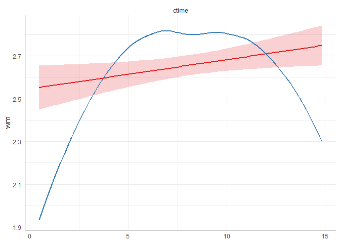
plot_model(mod2, 'pred') # hässlich

# schöner
sunday$pred_mod2 <- predict(mod2)
ggplot(sunday, aes(x = ctime, y = pred_mod2)) +
  geom_smooth(se = FALSE)
Random Slopes Modell
tmp <- poly(sunday$ctime, 2)
tmp <- as.data.frame(tmp)
names(tmp) <- c('poly1', 'poly2')
sunday <- cbind(sunday, tmp)
mod3a <- lmer(wm ~ 1 + poly1 + poly2 + (1 + poly1 | id), sunday)
mod3b <- lmer(wm ~ 1 + poly1 + poly2 + (1 + poly1 + poly2 | id), sunday)
anova(mod2, mod3a, mod3b, refit = FALSE)
## Data: sunday
## Models:
## mod2: wm ~ 1 + poly(ctime, 2) + (1 | id)
## mod3a: wm ~ 1 + poly1 + poly2 + (1 + poly1 | id)
## mod3b: wm ~ 1 + poly1 + poly2 + (1 + poly1 + poly2 | id)
##       npar    AIC    BIC  logLik deviance  Chisq Df
## mod2     5 2331.6 2356.4 -1160.8   2321.6
## mod3a    7 2242.3 2277.1 -1114.1   2228.3 93.299  2
## mod3b   10 2226.5 2276.3 -1103.3   2206.5 21.752  3
##       Pr(>Chisq)
## mod2
## mod3a  < 2.2e-16 ***
## mod3b  7.346e-05 ***
## ---
## Signif. codes:
## 0 '***' 0.001 '**' 0.01 '*' 0.05 '.' 0.1 ' ' 1
print(summ(mod3b))
## MODEL INFO:
## Observations: 1069
## Dependent Variable: wm
## Type: Mixed effects linear regression
##
## MODEL FIT:
## AIC = 2226.51, BIC = 2276.26
## Pseudo-R² (fixed effects) = 0.07
## Pseudo-R² (total) = 0.51
##
## FIXED EFFECTS:
## ---------------------------------------------------------
##                      Est.   S.E.   t val.     d.f.      p
## ----------------- ------- ------ -------- -------- ------
## (Intercept)          2.66   0.04    71.32   151.82   0.00
## poly1                2.38   1.00     2.37   151.94   0.02
## poly2               -6.32   0.73    -8.62   137.32   0.00
## ---------------------------------------------------------
##
## p values calculated using Satterthwaite d.f.
##
## RANDOM EFFECTS:
## ------------------------------------
##   Group      Parameter    Std. Dev.
## ---------- ------------- -----------
##     id      (Intercept)     0.40
##     id         poly1        9.81
##     id         poly2        5.18
##  Residual                   0.55
## ------------------------------------
##
## Grouping variables:
## -------------------------
##  Group   # groups   ICC
## ------- ---------- ------
##   id       148      0.34
## -------------------------
VarCorr(mod3b)
##  Groups   Name        Std.Dev. Corr
##  id       (Intercept) 0.39924
##           poly1       9.80970  -0.131
##           poly2       5.18308  -0.003 -0.498
##  Residual             0.55216
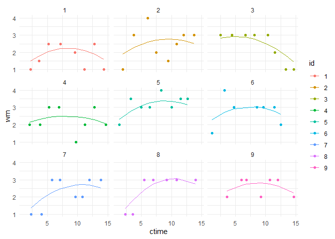
sunday$pred_mod3 <- predict(mod3b)

subset(sunday, as.numeric(id) < 10) |>
  ggplot(aes(x = ctime, y = wm, color = id)) +
    geom_point() +
    geom_line(aes(y = pred_mod3)) +
    theme_minimal() + facet_wrap(~ id)
Wachstumskurven mit Prädiktoren
- Dynamische Prädiktoren (L1-Prädiktoren)
- Variablen auf Ebene der Zeitpunkte
- Situationale Faktoren (z. B. Zeit, Ort, soziale Umgebung)
- Variable Personenfaktoren (z. B. Stimmung, wahrgenommener Stress)
- Erklären Abweichungen der Situationen vom generellen Trend
- Stabile Prädiktoren (L2-Prädiktoren)
- Variablen auf Ebene der Personen
- Generell stabile Merkmale (z. B. Geschlecht, Big 5, SES)
- Innerhalb der Erhebung unveränderliche Merkmale (z.B. Experimentalgruppe, Baselinemerkmale)
- Erklären interindividuelle Unterschiede (in der Veränderung)
Dynamische Prädiktoren
mod4 <- lmer(wm ~ 1 + poly1 + poly2 + pos + (1 + poly1 + poly2 | id), sunday)
## Warning in checkConv(attr(opt, "derivs"), opt$par, ctrl =
## control$checkConv, : Model failed to converge with
## max|grad| = 0.0045503 (tol = 0.002, component 1)
print(summ(mod4))
## MODEL INFO:
## Observations: 1069
## Dependent Variable: wm
## Type: Mixed effects linear regression
##
## MODEL FIT:
## AIC = 2223.53, BIC = 2278.25
## Pseudo-R² (fixed effects) = 0.08
## Pseudo-R² (total) = 0.51
##
## FIXED EFFECTS:
## ---------------------------------------------------------
##                      Est.   S.E.   t val.     d.f.      p
## ----------------- ------- ------ -------- -------- ------
## (Intercept)          2.62   0.04    67.35   184.38   0.00
## poly1                2.37   1.00     2.37   151.41   0.02
## poly2               -6.31   0.74    -8.58   136.09   0.00
## posja                0.14   0.05     3.06   950.08   0.00
## ---------------------------------------------------------
##
## p values calculated using Satterthwaite d.f.
##
## RANDOM EFFECTS:
## ------------------------------------
##   Group      Parameter    Std. Dev.
## ---------- ------------- -----------
##     id      (Intercept)     0.39
##     id         poly1        9.79
##     id         poly2        5.27
##  Residual                   0.55
## ------------------------------------
##
## Grouping variables:
## -------------------------
##  Group   # groups   ICC
## ------- ---------- ------
##   id       148      0.34
## -------------------------
sunday$pred_mod4 <- predict(mod4)

subset(sunday, as.numeric(id) < 10) |>
  ggplot(aes(x = ctime, y = wm, color = id)) +
    geom_point(aes(shape = pos)) +
    geom_line(aes(y = pred_mod4)) +
    theme_minimal() + facet_wrap(~ id)
Sonderfall discontinuous growth:
- L1-Prädiktoren können auch Kodiervariablen sein
- Übergang zwischen Grund- und Sekundarschule
- Interventionsbeginn
- Tagesübergänge
- Kodiervariablen können plötzliche Sprünge oder eine Veränderung des Wachstums ermöglichen
| time | event | ptime |
|---|---|---|
| 1 | 0 | 0 |
| 2 | 0 | 0 |
| 3 | 0 | 0 |
| 4 | 1 | 0 |
| 5 | 1 | 1 |
| 6 | 1 | 2 |
| 7 | 1 | 3 |
- “event”: plötzlicher Sprung im Niveau
- “ptime”: Veränderung der Trajectory
Stabile Prädiktoren
mod5 <- lmer(wm ~ 1 + poly1 + poly2 + meq + (1 + poly1 + poly2 | id), sunday) # + meq = additiver Effekt auf das Mittel (Interaktion morning/evening)
print(summ(mod5))
## MODEL INFO:
## Observations: 1069
## Dependent Variable: wm
## Type: Mixed effects linear regression
##
## MODEL FIT:
## AIC = 2236.90, BIC = 2291.62
## Pseudo-R² (fixed effects) = 0.07
## Pseudo-R² (total) = 0.51
##
## FIXED EFFECTS:
## ---------------------------------------------------------
##                      Est.   S.E.   t val.     d.f.      p
## ----------------- ------- ------ -------- -------- ------
## (Intercept)          2.69   0.16    16.63   153.33   0.00
## poly1                2.37   1.00     2.36   151.91   0.02
## poly2               -6.32   0.73    -8.62   137.25   0.00
## meq                 -0.00   0.01    -0.21   153.07   0.83
## ---------------------------------------------------------
##
## p values calculated using Satterthwaite d.f.
##
## RANDOM EFFECTS:
## ------------------------------------
##   Group      Parameter    Std. Dev.
## ---------- ------------- -----------
##     id      (Intercept)     0.40
##     id         poly1        9.81
##     id         poly2        5.19
##  Residual                   0.55
## ------------------------------------
##
## Grouping variables:
## -------------------------
##  Group   # groups   ICC
## ------- ---------- ------
##   id       148      0.35
## -------------------------
mod5b <- lmer(wm ~ 1 + poly1 + poly2 + meq + meq:poly2 + meq:poly1 + # kann meq weggelassen werden, wenn es nicht interessiert?
                (1 + poly1 + poly2 | id), sunday)
summ(mod5b)
| Observations | 1069 |
| Dependent variable | wm |
| Type | Mixed effects linear regression |
| AIC | 2232.68 |
| BIC | 2297.35 |
| Pseudo-R² (fixed effects) | 0.08 |
| Pseudo-R² (total) | 0.51 |
| Est. | S.E. | t val. | d.f. | p | |
|---|---|---|---|---|---|
| (Intercept) | 2.63 | 0.16 | 16.17 | 153.83 | 0.00 |
| poly1 | 17.34 | 4.23 | 4.09 | 156.44 | 0.00 |
| poly2 | -9.38 | 3.20 | -2.93 | 139.61 | 0.00 |
| meq | 0.00 | 0.01 | 0.20 | 153.70 | 0.85 |
| poly2:meq | 0.11 | 0.12 | 0.95 | 140.17 | 0.34 |
| poly1:meq | -0.56 | 0.15 | -3.63 | 156.41 | 0.00 |
| p values calculated using Satterthwaite d.f. |
| Group | Parameter | Std. Dev. |
|---|---|---|
| id | (Intercept) | 0.40 |
| id | poly1 | 9.21 |
| id | poly2 | 5.23 |
| Residual | 0.55 |
| Group | # groups | ICC |
|---|---|---|
| id | 148 | 0.34 |
Cross-Level-Interaktionen
mod6 <- lmer(wm ~ 1 + poly1*meq + poly2*meq + (1 + poly1 + poly2 | id), sunday)
print(summ(mod6))
## MODEL INFO:
## Observations: 1069
## Dependent Variable: wm
## Type: Mixed effects linear regression
##
## MODEL FIT:
## AIC = 2232.68, BIC = 2297.35
## Pseudo-R² (fixed effects) = 0.08
## Pseudo-R² (total) = 0.51
##
## FIXED EFFECTS:
## ---------------------------------------------------------
##                      Est.   S.E.   t val.     d.f.      p
## ----------------- ------- ------ -------- -------- ------
## (Intercept)          2.63   0.16    16.17   153.82   0.00
## poly1               17.34   4.23     4.10   156.47   0.00
## meq                  0.00   0.01     0.20   153.69   0.85
## poly2               -9.38   3.20    -2.93   139.60   0.00
## poly1:meq           -0.56   0.15    -3.63   156.43   0.00
## meq:poly2            0.11   0.12     0.95   140.17   0.34
## ---------------------------------------------------------
##
## p values calculated using Satterthwaite d.f.
##
## RANDOM EFFECTS:
## ------------------------------------
##   Group      Parameter    Std. Dev.
## ---------- ------------- -----------
##     id      (Intercept)     0.40
##     id         poly1        9.21
##     id         poly2        5.23
##  Residual                   0.55
## ------------------------------------
##
## Grouping variables:
## -------------------------
##  Group   # groups   ICC
## ------- ---------- ------
##   id       148      0.34
## -------------------------
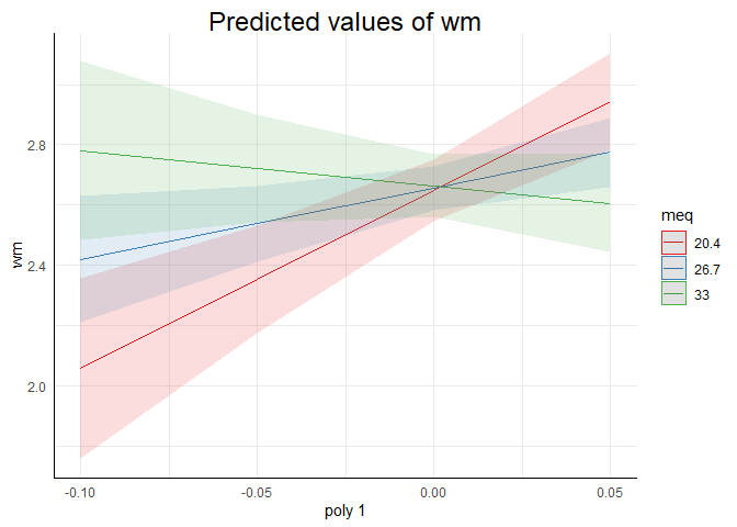
plot_model(mod6, 'pred', terms = c('poly1', 'meq'))
Autoregressive Modelle
- Beliebt weil Grundlage für Vektor-Autoregressive Modelle (Längsschnitt-Netzwerkanalysen)
- iid Annahme (independent and identically distributed)
- L1-Residuen sind voneinander unabhängig
- L1-Residuen folgen der gleichen Verteilung (impliziert Homoskedastizität)
- Annahmen der OLS Regression
- Unabhängigkeit der Residuen
- Homoskedastizität der Residuen
- MLM berücksichtigt nur Abhängigkeiten durch angegebene Cluster-Variablen
- Andere Abhängigkeiten (serielle Abhängigkeit, weitere Clusterungsebenen, usw.) können weiterhin zu Verzerrungen führen
Explizite Autoregression
- Lag Variable erstellen
# mit basis R-Befehlen
sunday$wm_lag <- NA
for (i in sunday$id) {
  sunday[sunday$id == i, 'wm_lag'] <- embed(c(NA, sunday[sunday$id == i, 'wm']), 2)[, 2]
}

# mit dplyr (sehr verbreitet)
library(dplyr)
sunday <- group_by(sunday, id) %>% mutate(wm_lag = lag(wm))
mod0 <- lmer(gs ~ 1 + (1 | id), sunday)
mod1 <- lmer(gs ~ 1 + gs_lag + (1 | id), sunday)
anova(mod0, mod1)
## Error in anova.merMod(mod0, mod1): models were not all fitted to the same size of dataset
mod0b <- update(mod0, data = mod1@frame)
mod1b <- update(mod1, data = mod1@frame)
anova(mod0b, mod1b)
## refitting model(s) with ML (instead of REML)
## Data: mod1@frame
## Models:
## mod0b: gs ~ 1 + (1 | id)
## mod1b: gs ~ 1 + gs_lag + (1 | id)
##       npar    AIC    BIC  logLik deviance  Chisq Df
## mod0b    3 1189.9 1204.4 -591.95   1183.9
## mod1b    4 1078.8 1098.1 -535.38   1070.8 113.13  1
##       Pr(>Chisq)
## mod0b
## mod1b  < 2.2e-16 ***
## ---
## Signif. codes:
## 0 '***' 0.001 '**' 0.01 '*' 0.05 '.' 0.1 ' ' 1
Drei Varianzkomponenten:
- Stabiler Anteil (ICC)
- Vorhersagbare State-Komponente
- Unvorhersagbare State-Komponente
MuMIn::r.squaredGLMM(mod0b)
##      R2m       R2c
## [1,]   0 0.4405919
MuMIn::r.squaredGLMM(mod1b)
##            R2m       R2c
## [1,] 0.2419568 0.3217569
print(summ(mod1b))
## MODEL INFO:
## Observations: 921
## Dependent Variable: gs
## Type: Mixed effects linear regression
##
## MODEL FIT:
## AIC = 1090.18, BIC = 1109.49
## Pseudo-R² (fixed effects) = 0.24
## Pseudo-R² (total) = 0.32
##
## FIXED EFFECTS:
## --------------------------------------------------------
##                     Est.   S.E.   t val.     d.f.      p
## ----------------- ------ ------ -------- -------- ------
## (Intercept)         1.59   0.09    17.60   367.60   0.00
## gs_lag              0.47   0.03    16.02   407.11   0.00
## --------------------------------------------------------
##
## p values calculated using Satterthwaite d.f.
##
## RANDOM EFFECTS:
## ------------------------------------
##   Group      Parameter    Std. Dev.
## ---------- ------------- -----------
##     id      (Intercept)     0.14
##  Residual                   0.41
## ------------------------------------
##
## Grouping variables:
## -------------------------
##  Group   # groups   ICC
## ------- ---------- ------
##   id       148      0.11
## -------------------------
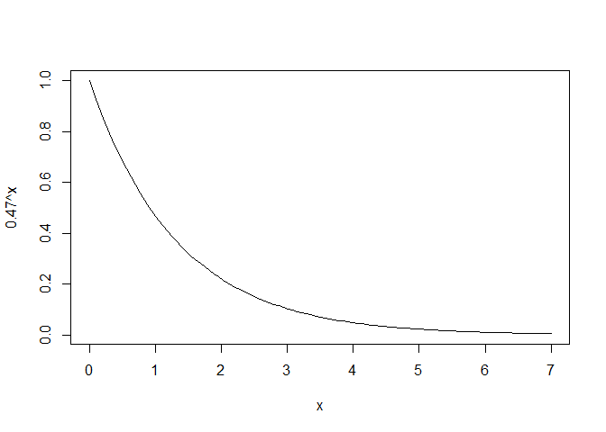
Serielle Abhängigkeit: $$ y_{ti} = \gamma_{00} + \gamma_{10} y_{(t-1)i} + u_{0i} + r_{ti} \ y_{(t-1)i} = \gamma_{00} + \gamma_{10} y_{(t-2)i} + u_{0i} + r_{(t-1)i} \ $$
Indirekter Effekt: $\beta_{t(t-\text{lag})} = \gamma_{10}^{\text{lag}}$
curve(.47^x, xlim = c(0, 7))
- Vorteile expliziter AR:
- Einfache Spezifikation und Interpretation
- Umgeht die Unabhängigkeitsannahme
- Erlaubt Zufallseffekte der Autoregression
- Nachteile expliziter AR:
- Nimmt zusätzliche Prädiktoren in die Gleichung auf
- Erste Messung pro Person entfällt durch Missing
- Nimmt gleiche Abstände zwischen Messungen an
- Interpretation der Parameter immer unter Annahme gleicher Werte zum vorherigen Zeitpunkt
Autoregressive Fehlerstruktur
- Ohne zusätzlichen Prädiktoren
- Residualkovarianzmatrix wird verändert
- Gleiche Idee: ein Parameter ($\rho$) bezeichnet die zusätzliche Abhängigkeit zwischen benachbarten Messungen
- Voraussetzung ist hier, dass der autoregressive Effekte positiv ist
$$ \Sigma_{r} = var(r_{ti}) \begin{bmatrix} 1 & \rho & \rho^2 & \rho^3 \ \rho & 1 & \rho & \rho^2 \ \rho^2 & \rho & 1 & \rho \ \rho^3 & \rho^2 & \rho & 1 \end{bmatrix} $$
- lme4 dazu nicht in der Lage
- viele alternative Pakete können verschiedene Residualstrukturen
- hier Awendung mit
nlme, weil vorinstalliert undlme4relativ ähnlich
library(nlme)
##
## Attaching package: 'nlme'
## The following object is masked from 'package:lme4':
##
##     lmList
## The following object is masked from 'package:dplyr':
##
##     collapse
mod0_nlme <- lme(fixed = gs ~ 1, random = ~ 1 | id, data = sunday)
summary(mod0_nlme)
## Linear mixed-effects model fit by REML
##   Data: sunday
##        AIC      BIC    logLik
##   1386.189 1401.109 -690.0943
##
## Random effects:
##  Formula: ~1 | id
##         (Intercept)  Residual
## StdDev:   0.3489966 0.4055539
##
## Fixed effects:  gs ~ 1
##                Value  Std.Error  DF  t-value p-value
## (Intercept) 3.001416 0.03132548 921 95.81391       0
##
## Standardized Within-Group Residuals:
##           Min            Q1           Med            Q3
## -5.5913005031 -0.4191647703 -0.0005044242  0.4940976394
##           Max
##  2.5971130291
##
## Number of Observations: 1069
## Number of Groups: 148
summary(mod0)
## Linear mixed model fit by REML. t-tests use
##   Satterthwaite's method [lmerModLmerTest]
## Formula: gs ~ 1 + (1 | id)
##    Data: sunday
##
## REML criterion at convergence: 1380.2
##
## Scaled residuals:
##     Min      1Q  Median      3Q     Max
## -5.5913 -0.4192 -0.0005  0.4941  2.5971
##
## Random effects:
##  Groups   Name        Variance Std.Dev.
##  id       (Intercept) 0.1218   0.3490
##  Residual             0.1645   0.4056
## Number of obs: 1069, groups:  id, 148
##
## Fixed effects:
##              Estimate Std. Error        df t value Pr(>|t|)
## (Intercept)   3.00142    0.03133 145.15591   95.81   <2e-16
##
## (Intercept) ***
## ---
## Signif. codes:
## 0 '***' 0.001 '**' 0.01 '*' 0.05 '.' 0.1 ' ' 1
mod1_nlme <- lme(fixed = gs ~ 1, random = ~ 1 | id, data = sunday,
  correlation = corAR1())
summary(mod1_nlme)
## Linear mixed-effects model fit by REML
##   Data: sunday
##        AIC     BIC    logLik
##   1296.226 1316.12 -644.1131
##
## Random effects:
##  Formula: ~1 | id
##         (Intercept) Residual
## StdDev:   0.3021535 0.442272
##
## Correlation Structure: AR(1)
##  Formula: ~1 | id
##  Parameter estimate(s):
##       Phi
## 0.3919874
## Fixed effects:  gs ~ 1
##                Value  Std.Error  DF  t-value p-value
## (Intercept) 2.996439 0.03125952 921 95.85685       0
##
## Standardized Within-Group Residuals:
##         Min          Q1         Med          Q3         Max
## -5.09726494 -0.35562195  0.00323874  0.47579376  2.39482725
##
## Number of Observations: 1069
## Number of Groups: 148
- Das correlation-Argument erlaubt die Spezifikation einer Korrelationsstruktur auf L1
corAR1()wählt die autoregressive Struktur 1. Ordnung- Es wird angenommen, dass die Daten richtig sortiert sind!
Zeitkontinuierliche Autoregression
- Bisherige Annahme: gleiche Abstände der Messungen, gleiche Messungen für alle Personen
- $\phi$ bzw. $\gamma_{10}$ beschreiben AR zwischen $t$ und $t-1$ (diskrete Zeitpunkte)
- $\phi$ berücksichtigt dabei nicht zeitlichen Abstand zwischen $t$ und $t-1$
mod2_nlme <- lme(fixed = gs ~ 1, random = ~ 1 | id, data = sunday,
  correlation = corCAR1(, form = ~ ctime))
summary(mod2_nlme)
## Linear mixed-effects model fit by REML
##   Data: sunday
##        AIC     BIC    logLik
##   1289.736 1309.63 -640.8678
##
## Random effects:
##  Formula: ~1 | id
##         (Intercept)  Residual
## StdDev:   0.3072518 0.4405892
##
## Correlation Structure: Continuous AR(1)
##  Formula: ~ctime | id
##  Parameter estimate(s):
##       Phi
## 0.5690876
## Fixed effects:  gs ~ 1
##                Value  Std.Error  DF  t-value p-value
## (Intercept) 2.997053 0.03133165 921 95.65577       0
##
## Standardized Within-Group Residuals:
##          Min           Q1          Med           Q3
## -5.138995611 -0.379382642  0.002754803  0.480001652
##          Max
##  2.405839942
##
## Number of Observations: 1069
## Number of Groups: 148
- $\phi$ hier interpretieren als AR über eine Stunde
- In diskretem Fall: AR zwischen zwei Zeitpunkten
- Mittlerer Abstand zwischen zwei Zeitpunkten: 1.79
- Annäherung: $.569^{1.79} = 0.365$ (aus Ergebnis oben: $\phi = .392$)