Introduction

Longitudinal network analysis (LNA) in psychology focuses on examining how psychological variables—often conceptualized as nodes in a network—interact and evolve within individuals over time. Traditional research in psychology has relied heavily on cross-sectional or between-person methods to draw conclusions about within-person processes. However, as researchers have become increasingly interested in individualized patterns of change (e.g., how a single person’s symptoms, behaviors, or cognitive states influence each other over time), it has become clear that more nuanced longitudinal methods are needed.

This chapter provides an overview of common analytical approaches in psychological research, emphasizes the dangers of misusing cross-sectional and between-person methods when investigating within-person questions, and introduces key concepts—such as the ecological fallacy, and ergodicity—that are crucial for understanding how to appropriately conduct and interpret longitudinal (including network) analyses in psychology.

Analytical Approaches in Psychology

In psychological research, various analytical approaches are employed to understand the complexities of human behavior and mental processes. Each method offers unique insights by focusing on different levels of data analysis. Below is an expanded overview of these approaches, emphasizing their applications, advantages, and limitations.

1. Cross-Sectional Analysis

Description: Cross-sectional analysis examines data from multiple individuals at a single point in time. It provides a “snapshot” of a population, revealing correlations or associations between variables measured simultaneously.

Example: A study assessing the correlation between depressive symptoms and anxiety levels among patients diagnosed with major depressive disorder at a specific clinic visit. The analysis might reveal a positive correlation, indicating that higher levels of depressive symptoms are associated with increased anxiety at that time.

Advantages:

• Efficient for identifying associations between variables.
• Relatively quick and cost-effective, as data is collected once.

Limitations:

• Cannot establish causality due to the simultaneous measurement of variables.
• Unable to distinguish between within-person (intra-individual) and between-person (inter-individual) effects.

In this semester: We have learned Regression (Thatcher et al., 2023) and Logistic Regression (Lin et al., 2023), both of which are commonly used in cross-sectional studies. These methods help us assess the association between predictor variables (e.g., symptoms, demographic factors) and outcomes (e.g., diagnostic status, behavioral scores) in a dataset collected at one specific time point.

2. Between-Person Analysis (in the strictest sense)

Description: Between-person analysis focuses on examining differences between individuals by analyzing stable traits or average behaviors over time. This method investigates how individuals vary from one another concerning certain characteristics.

Example: Analyzing whether patients who, on average, report higher levels of childhood trauma also exhibit higher average levels of post-traumatic stress disorder (PTSD) symptoms across multiple assessments.

Advantages:

• Highlights stable individual differences.
• Useful for identifying traits that distinguish individuals within a population.

Limitations:

• Does not account for fluctuations within an individual over time.
• May miss contextual or situational factors affecting behavior.

In this semester: We have explored Cluster-Mean Effects in Linear Mixed Models (LMM) (Liu et al., 2024), which allow us to model and interpret between-person differences. By including cluster-mean predictors, we can investigate how an individual’s average level of a variable relates to their outcomes compared to others in the sample.

3. Within-Person Analysis (in the strictest sense)

Description: Within-person analysis (in the strictest sense) focuses on the variation of behaviors or responses within the same individual over time. By tracking how a person changes from moment to moment (or day to day, week to week, etc.), this approach isolates factors that directly influence an individual’s behavior or state.

Example: Monitoring a specific patient’s daily mood fluctuations and stress levels to determine if increased stress on a particular day correlates with a subsequent decrease in mood for that individual.

Advantages:

• Captures dynamic, time-varying changes within the same person.
• Isolating purely intra-individual effects.

Limitations:

• Findings may not generalize to other individuals.
• Requires repeated measurements, which can be resource-intensive.

In this semester: We covered Random Slopes in Linear Mixed Models (LMM) (Liu et al., 2024), which are essential for within-person analyses. Random slopes allow each individual in a study to have a unique relationship between predictor variables and outcomes over time, thereby highlighting personalized patterns.

4. Fixed-Effects Analysis

Description: Fixed-effects analysis looks at within-person relationships across a sample by modeling how day-to-day or time-to-time changes in variables co-occur, essentially capturing the effect of a predictor on an outcome within a “hypothetical average person” in that sample.

Example: Determining whether, on days when individuals in a clinical sample experience higher-than-their-own-average stress levels, they also tend to report higher-than-their-own-average severity of obsessive-compulsive symptoms. These relationships reflect the pattern of a hypothetical “average” person, rather than any specific individual in the sample.

Advantages:

• Controls for unobserved individual characteristics that do not change over time.
• Provides insights into causal relationships within individuals.

Advantages:

• Controls for unobserved individual characteristics that do not change over time, by focusing on within-person variations across the sample.
• Provides insights into relationships at the within-person level, reflecting patterns observed in a hypothetical “average” person rather than in specific individuals.

Limitations:

• Cannot examine effects of variables that do not change over time, as these are constant within individuals and thus controlled out in the analysis.
• The results do not represent the unique patterns of any specific individual, as they reflect aggregated within-person effects across the sample.

Important: In within-person analysis, the focus is on a specific individual, analyzing how their behavior or responses vary over time. In contrast, fixed-effects analysis aggregates data across individuals to estimate average within-person effects, essentially modeling the behavior of a hypothetical “average” person. This distinction is crucial: while within-person analysis provides insights into individual-specific processes, fixed-effects analysis offers a generalized view.

In this semester: We studied ANCOVA with Mean-Centered Variables (Schleider et al., 2022) and Fixed-Effects Models in Linear Mixed Models (LMM) (Liu et al., 2024). These approaches help isolate how fluctuations in predictor variables within individuals (over time) relate to fluctuations in outcomes, while controlling out all stable, time-invariant differences across people.

Misuse of Analyses in Psychology

Despite the wide availability of methods tailored to within-person questions, it remains common for researchers (especially in psychopathology) to rely on cross-sectional or between-person analyses to address within-person hypotheses. This practice can lead to misleading conclusions—what appears to be true at the group level may not apply to any single individual.

Example: Sleep Quality and Anxiety

In traditional psychopathology research, a common approach to understanding the relationship between sleep quality and anxiety involves cross-sectional analysis. Researchers might pose a clinical question such as, “Does improving sleep quality reduce anxiety levels?” To explore this, they conduct a survey at a single time point, collecting data from a large sample of participants. This approach aligns with the principle that a larger sample size enhances the reliability of findings. Through correlation analysis, they may discover a negative correlation between sleep quality and anxiety, indicating that better sleep quality is associated with lower anxiety levels. This constitutes a cross-sectional analysis, as it examines data from multiple individuals at one specific point in time.

To strengthen the evidence, researchers might replicate the study across multiple time points, each time collecting data from different participants. By consistently finding similar negative correlations between sleep quality and anxiety, they perform a between-person analysis. This approach focuses on differences between individuals, examining how variations in sleep quality correlate with anxiety levels across different people. Such reproducibility is a hallmark of robust scientific research.

As psychologists, we are particularly interested in understanding effects within individuals. However, traditional approaches in psychopathology have often misused analytical methods when addressing this goal. Specifically, cross-sectional analysis and between-person analysis—though commonly employed—are not designed to answer questions about within-person processes. These methods focus on identifying associations between variables across individuals or at single time points, which can lead to misleading conclusions when used to infer causal relationships within individuals.

For example, cross-sectional studies might show a negative correlation between sleep quality and anxiety at a single time point across a large sample. While this suggests that people with better sleep tend to report lower anxiety, it does not tell us whether improving sleep in a specific individual will reduce their anxiety. Similarly, between-person analyses compare average differences between individuals, such as whether people who generally sleep better tend to be less anxious. However, these between-person differences do not necessarily reflect how changes in sleep affect anxiety within the same person over time. This phenomenon is known as the ecological fallacy, where relationships observed at the group level are incorrectly assumed to apply to individuals.

To truly understand within-person effects, we need to employ within-person analysis, which examines how changes within an individual over time affect outcomes. For instance, we might ask, “Can we determine the anxiety treatment effect for a specific patient after a sleep quality intervention?” To answer this, we would monitor an individual’s sleep quality and anxiety levels over time, assessing whether improvements in their sleep correspond to reductions in their anxiety. This approach allows us to observe causal relationships within that person and tailor interventions based on their unique experiences.

Additionally, fixed-effects analysis offers a way to generalize within-person findings across individuals. Rather than focusing on between-person differences, fixed-effects models analyze within-person variations while controlling for stable, time-invariant individual characteristics. This enables us to answer questions like, “Can we predict the anxiety treatment effect for any future individual receiving a sleep quality intervention?” By examining how changes in sleep quality within individuals are associated with changes in anxiety, we can estimate the average within-person treatment effect—essentially modeling the effects for a hypothetical “average” person. This is valuable for making evidence-based treatment predictions while acknowledging individual variability.

In summary, the misuse of cross-sectional and between-person analyses has led to incorrect assumptions about individual-level effects in psychopathology research. To apply findings effectively in clinical practice, within-person and fixed-effects analyses are essential. They provide the necessary insights to understand how interventions impact individuals over time, moving beyond broad associations to inform personalized treatment strategies and more accurate predictions for future patients.

Highlighting Within- and Between-Person Differences

The distinction between within-person and between-person effects is fundamental in psychological research, as it addresses how relationships between variables can differ when analyzed at the individual level versus the group level. A classic illustration of this distinction is provided by Epskamp et al. (2018), building upon an example by Hamaker (2012).

Consider the relationship between typing speed and the number of spelling errors. At the within-person level, for a specific individual, an increase in typing speed beyond their usual pace may lead to more spelling errors. This suggests a positive within-person relationship: as an individual types faster than their average speed, they tend to make more errors.

Conversely, at the between-person level, when comparing different individuals, those who type faster on average may actually make fewer spelling errors. This could be because individuals who consistently type quickly are often more experienced typists and thus more accurate, leading to a negative between-person relationship: faster typists tend to make fewer errors.

This scenario exemplifies what is often referred to as Simpson’s Paradox, where a trend observed within individual groups reverses when these groups are combined. In this case, the within-person positive relationship contrasts with the between-person negative relationship. Understanding this paradox is crucial, as it highlights that relationships observed at the group level may not necessarily apply at the individual level, and vice versa.

Recognizing the distinction between within-person and between-person effects has significant implications for both research and practical interventions. For instance, if an individual aims to reduce their spelling errors, they might consider slowing down their typing speed, as their personal data indicates a positive relationship between speed and errors. However, advising all individuals to type quicker based on between-person data could be misguided, especially for those who are proficient typists and do not exhibit the same within-person relationship.

Ergodicity in Psychological Research

In psychological research, understanding the distinction between within-person and between-person effects is crucial. A key concept that addresses when these effects might align is ergodicity.

Ergodicity is a principle derived from statistical mechanics. When applied to psychological processes, it implies that statistical characteristics observed across individuals (between-person effects) would be equivalent to those observed within an individual over time (within-person effects). For this equivalence to hold, two stringent conditions must be met:

1. Stationarity: The process must be stationary, meaning that its statistical properties, such as mean and variance, remain constant over time. In psychological terms, this would require that an individual’s behavior and experiences do not change over time—a condition rarely met in reality.

2. Homogeneity: The individuals within the population must be homogeneous, indicating that each person is virtually identical in terms of the process being studied. This implies that all individuals respond to stimuli or interventions in the same way, without individual differences.

These assumptions are so strong that they are unlikely to hold in psychological research over long periods. Human behavior is inherently dynamic and influenced by various internal and external factors, leading to deviations from strict stationarity. While short-term stationarity may be a reasonable assumption in some contexts, maintaining stability over extended periods is challenging and rarely observed in practice. Additionally, individual differences are a cornerstone of psychological science, making the assumption of homogeneity impractical.

Implications for Research Methodology

Given the improbability of ergodicity in psychological processes, relying solely on cross-sectional data to infer within-person dynamics can be misleading. As Molenaar (2004) argued, the common practice of using cross-sectional results to uncover general laws assumed to apply to each individual is unfounded. This is because cross-sectional analyses capture between-person variability at a single time point and do not account for the temporal dynamics within individuals.

To better understand causal relationships and within-person effects, researchers should consider methodologies that involve intensive time-series data or panel data:

• Intensive Time-Series Data: This approach involves measuring several subjects on many occasions, allowing for the analysis of intra-individual variability and the examination of how processes unfold over time within individuals.

• Panel Data: This method entails measuring many people on only a few occasions, providing a balance between capturing individual dynamics and maintaining a broader sample.

By employing these methodologies, researchers can more accurately capture the complexities of psychological processes and avoid the pitfalls associated with assuming ergodicity.

Study

Having laid out the conceptual foundations of cross-sectional, between-person, within-person, and fixed-effects approaches—and having discussed why distinguishing these levels of analysis is vital—we now turn to a concrete application within psychopathology research. This chapter section explores a study by Lunansky et al. (2023) that investigates how affect regulation contributes to the onset and course of depressive complaints. Their work exemplifies how longitudinal and network-based methodologies can clarify complex, dynamic processes that underlie mental health conditions.

Affect Regulation and Depression

Major Depression (MD) is one of the leading causes of non-fatal health loss globally, impairing quality of life and daily functioning. Despite the substantial body of research, understanding precisely how depressive symptoms develop and change over time remains challenging. One key complication is the heterogeneity of depressive experiences: individuals with the same diagnosis can exhibit substantially different symptom profiles and trajectories.

The role of affect has emerged as a critical factor in explaining these variations. Affect encompasses both positive affect (PA) (e.g., feeling inspired, enthusiastic) and negative affect (NA) (e.g., feeling scared, upset). Each plays a unique role in stress responsiveness and emotional well-being:

• Negative Affect (NA): Characterized by emotions such as fear or upset. Individuals with heightened NA in response to stress are at greater risk for both the onset and persistence of depressive symptoms. Chronic stress exposure—or a dysregulated response to it—can lead to a more pervasive perception of threat, fueling the development or maintenance of depressive complaints.

• Positive Affect (PA): Encompasses states like inspiration, excitement, and determination. High PA acts as a buffer against stress, reducing physiological arousal (e.g., on cardiovascular or inflammatory systems) and thus mitigating the risk of depressive outcomes.

• Interplay Between PA and NA: The combined effect of PA and NA may not be as simple as the sum of each component; rather, they function as dynamically interconnected aspects of emotional life. Understanding how these two affective dimensions interact over time—within individuals—offers deeper insight into why depressive symptoms emerge and persist for some people but not for others. This is the reason why we need network approach to explore all variables together.

Study Objectives and Hypotheses

In their paper “Disentangling the Role of Affect in the Evolution of Depressive Complaints Using Complex Dynamical Networks,” Lunansky et al. (2023) aimed to examine the dynamic links between affect and depression. The research objectives spanned multiple analytical levels, reflecting different analysis frameworks introduced in previous chapters:

1. Exploration of Affect Individual Difference (Between-Person Analysis): Investigate how patterns of increasing or decreasing positive affect (PA) and negative affect (NA) across participants relate to changes in depressive complaints over time. This between-person focus highlights whether individuals with generally rising NA (or falling PA) tend to show worsening depressive symptoms compared to other participants.

2. Exploration of Affect Trajectories (Fixed-Effects Analysis): Examine the direct interplay between affect and depressive complaints within a “hypothetical average individual,” while controlling for time-invariant personal characteristics. Using a fixed-effects approach helps isolate how fluctuations in PA and NA (relative to each person’s own average) co-occur with changes in depressive symptoms, removing confounds that remain constant over time (e.g., stable personality traits).

3. Investigation of Person-Specific Network Density: Assess how individual differences in the connectivity (i.e., “density”) of affective networks relate to changes in depressive complaints. If an individual has a highly interconnected network—where activating one symptom or affective state strongly influences others—this may predispose them to more persistent or severe depressive episodes. High network density could mean that small fluctuations in NA or PA rapidly cascade through one’s emotional and symptomatic system, like we have learned in the last part.

Study design

The study was conducted during the initial wave of the COVID-19 pandemic, providing a unique context to examine affect regulation under prolonged stress:

• Participants: Data were collected from March 20th, 2020, to August 5th, 2020. Participants completed the Positive and Negative Affect Schedule (PANAS) to assess PA and NA, and the Patient Health Questionnaire-9 (PHQ-9) to measure depressive symptoms.

• Measurement Intervals: A clear three-day response interval was identified, dividing the total study period into 33 three-day measurement occasions.

• Final Sample: The final sample included participants who provided data for at least 20 occasions, resulting in 228 individuals with data spanning 20 to 33 occasions over 9 to 14 weeks.

The dataset utilized in this study is publicly available and can be accessed via the Open Science Framework (OSF) at the following link: https://osf.io/2zh4f/

You can also find the dataset in the Moodle platform.

load("COVID19_dynamic_analyses_cleaned.Rdata")

colnames(data)[5:22] <- c("Insp", "Alert", "Exc", "Ent", 
                          "Det","Afraid", "Upset", "Nervous", 
                          "Scared", "Dist", "LoI", "DepMood", 
                          "SleepDis", "Fatigue", "Appet", 
                          "Worth", "Con", 
                          "PsychMot")

head(data)

##   sub_id measurement measurement_date     PHQ9 Insp Alert Exc Ent Det Afraid Upset Nervous Scared Dist       LoI
## 1      1           1       2020-03-21      NaN  NaN   NaN NaN NaN NaN    NaN   NaN     NaN    NaN  NaN       NaN
## 2      1           2       2020-03-24 6.666667    1   2.0   1 1.0   1      1     1       1      1  1.0 0.6666667
## 3      1           3       2020-03-27 6.500000    1   1.5   1 1.5   1      1     1       1      1  1.5 1.0000000
## 4      1           4       2020-03-30 6.000000    1   1.0   1 2.0   2      1     2       1      2  2.0 1.0000000
## 5      1           5       2020-04-02 4.000000    1   2.0   2 2.0   2      2     2       2      2  2.0 0.0000000
## 6      1           6       2020-04-05      NaN  NaN   NaN NaN NaN NaN    NaN   NaN     NaN    NaN  NaN       NaN
##   DepMood SleepDis Fatigue Appet     Worth Con  PsychMot  group    change
## 1     NaN      NaN     NaN   NaN       NaN NaN       NaN switch no_change
## 2       1        1       1     1 0.3333333   1 0.6666667 switch no_change
## 3       1        1       1     1 0.5000000   1 0.0000000 switch no_change
## 4       1        1       1     1 0.0000000   1 0.0000000 switch no_change
## 5       0        1       1     1 0.0000000   1 0.0000000 switch no_change
## 6     NaN      NaN     NaN   NaN       NaN NaN       NaN switch no_change

Within the loaded data object, key variables include:

• sub_id: Unique participant identifier.

• measurement: Index of each three-day measurement occasion.

• measurement_date: Date of each measurement.

• PHQ9: Summarized depression score at each measurement.

• PANAS variables: Multiple items (e.g., Exc, Alert).

• depression variables : Item-level depressive symptoms (e.g., DepMood, Fatigue)

any other variables we will not use in this part.

Longtidutinal Network as Vector Autoregression

In previous chapters, we emphasized the importance of within-person analyses and fixed effect analyses to capture how psychological processes evolve for the same individual across time. Traditional cross-sectional or between-person approaches often fail to illuminate the temporal dependencies inherent in psychological phenomena (e.g., how one day’s mood affects the next). A key extension of longitudinal methods is longitudinal network analysis (LNA), wherein multiple variables—such as mood, stress, or fatigue—are modeled as an interconnected system evolving over time.

Multilevel Regression with Autocorrelation

In longitudinal psychological research, data are collected repeatedly from the same individuals, resulting in a nested structure, where multiple observations are linked to the same person. In previous chapters, we introduced multilevel modeling (MLM) as a key method for handling such hierarchical data. However, beyond accounting for inter-individual variability, longitudinal studies must also consider autocorrelation, a crucial feature of repeated measures data.

Autocorrelation: Definition and Importance

Autocorrelation (or auto-regression, serial correlation) occurs when observations within an individual are correlated across adjacent time points. In other words, an individual’s score on a given psychological measure at one time point is often correlated with their score at a previous time point. This occurs because psychological and behavioral processes evolve gradually rather than changing randomly from one moment to the next.

For example, a person’s depressive symptoms today are likely influenced by their depressive symptoms yesterday. Similarly, stress levels in the morning may predict stress levels in the evening, as emotional states tend to persist over short periods.

This persistence creates a statistical dependency between repeated observations, violating the assumption of independence that many traditional models rely on. Ignoring autocorrelation in longitudinal data can lead to biased parameter estimates, underestimated standard errors, and invalid significance tests. This means that models failing to account for autocorrelation may falsely detect or fail to detect meaningful relationships.

In psychology, the most common form is Lag-1 Autocorrelation (First-Order Autocorrelation), where each observation is correlated only with the immediately preceding time point.

Incorporate Autocorrelation into MLM

To account for autocorrelation, we use Multilevel Regression with Autocorrelation, in which each variable is modeled as a function of its own past values (lagged predictors).

Let’s consider a scenario where $y$ represents Depressed Mood over time.

A simple first-order autoregressive model can be written as:

$$y_{ti}={\beta }_0+{\beta }_1{y}_{t-1,i}+{ϵ}_{ti}$$

where:

• $y_{ti}$ = Depressed Mood for individual$i$ at time$t$,
• $y_{t-1,i}$ = Depressed Mood at the previous time point,
• ${\beta }_0$ = Intercept (baseline level of depression),
• ${\beta }_1$ = Autoregressive coefficient (effect of past depression on current depression),
• ${ϵ}_{ti}$ = Residual error.

In this simplified model, each individual is assumed to have the same autoregressive effect (${\beta }_1$). However, individuals may differ in how persistent (or stable) their depressive symptoms are. To relax this assumption, we can introduce random slopes, allowing each individual to have their own autoregressive effect (${\beta }_{1i}$):

$${\beta }_{1i}={\gamma }_1+u_{1i}$$

where:

• ${\gamma }_1$ = Overall (fixed) autoregressive effect,
• $u_{1i}$ = Person-specific deviation from the average autoregression.

This random-slope model accounts for the fact that depressive symptoms may persist more strongly for some individuals than for others. For example:

• Some individuals may show high stability in depressive symptoms (${\beta }_{1i}\approx 0.9$, meaning symptoms persist strongly over time).
• Others may have lower stability (${\beta }_{1i}\approx 0.4$, meaning symptoms fluctuate more frequently). By allowing individual variability, we can better understand why and how people differ in their symptom trajectories over time.

Vector Autoregression (VAR)

Psychological variables rarely operate in isolation. Depressive mood may coexist with stress, fatigue, anxiety, or other symptoms in complex dynamical systems. By measuring multiple variables over time and analyzing their mutual influences, researchers gain a richer understanding of how psychological processes unfold and interact.

Vector Autoregression (VAR) is a multivariate extension of single-variable autoregressive models. Instead of modeling one outcome variable at a time, VAR treats multiple variables as endogenous (i.e., they can influence each other) in a system of equations. Each variable is regressed on lagged values of both itself and the other variables in the model.

Consider a scenario with two variables (most simple case, Bivariate example):$y$ (e.g., Depressed Mood) and $z$ (e.g., Fatigue). In a multilevel VAR(1) framework (first-order), each variable at time $t$ depends on its own value and the other variable’s value at time $t-1$.

Depressed Mood as the Dependent Variable

The model can be written as: Level 1 (Within-Person):

$$y_{ti}={\beta }_{0i}+{\beta }_{11,i}{y}_{t-1,i}+{\beta }_{12,i}{z}_{t-1,i}+{ϵ}_{y,t,i}$$

Where:

• $y_{ti}$: Depressed Mood for individual$i$ at time$t$.
• ${\beta }_{0i}$: Person-specific intercept for Depressed Mood.
• ${\beta }_{11,i}$: Autoregressive effect of past Depressed Mood ($y$ at$t-1$).
• ${\beta }_{12,i}$: Cross-lagged effect of past Fatigue ($z$ at$t-1$).
• ${ϵ}_{y,t,i}$: Person-specific residual error for$y$.

This equation suggests that:

• A person’s current mood depends partly on their past mood (autocorrelation).
• A person’s fatigue yesterday might predict depressed mood today (cross-lag effect).

Level 2 (Between-Person):

$$\begin{array}{rlrl}{\beta }_{0i}& ={\gamma }_{00}+u_{0i}{\beta }_{11,i}& ={\gamma }_{11}+u_{11,i}{\beta }_{12,i}& ={\gamma }_{12}+u_{12,i}\end{array}$$

Where:

• ${\gamma }_{00}$: Overall intercept across individuals.
• ${\gamma }_{11}$: Average (fixed) autoregressive effect of$y$ across individuals.
• ${\gamma }_{12}$: Average (fixed) cross-lagged effect of$z$ on$y$ across individuals.
• $u_{0i},u_{11,i},u_{12,i}$: Random effects capturing individual deviations from the average (fixed) effects.

Fatigue as the Dependent Variable

Now, let’s reverse the focus: instead of predicting mood, we predict fatigue using past fatigue and mood. In other words, Fatigue is the Dependent Variable.

The model can be written as: Level 1 (Within-Person):

$$z_{ti}={\beta }_{0i}+{\beta }_{22,i}{z}_{t-1,i}+{\beta }_{21,i}{y}_{t-1,i}+{ϵ}_{z,t,i}$$

Where:

• $z_{ti}$: Fatigue for individual$i$ at time$t$.
• ${\beta }_{0i}$: Person-specific intercept for Fatigue.
• ${\beta }_{22,i}$: Autoregressive effect of past Fatigue ($z$ at$t-1$).
• ${\beta }_{21,i}$: Cross-lagged effect of past Depressed Mood ($y$ at$t-1$).
• ${ϵ}_{z,t,i}$: Person-specific residual error for$z$.

This equation suggests that:

• A person’s fatigue today is influenced by their fatigue yesterday (autocorrelation).
• A person’s depressed mood yesterday may predict fatigue today (cross-lag effect).

Level 2 (Between-Person):

$$\begin{array}{rlrl}{\beta }_{0i}& ={\gamma }_{00}+u_{0i}{\beta }_{22,i}& ={\gamma }_{22}+u_{22,i}{\beta }_{21,i}& ={\gamma }_{21}+u_{21,i}\end{array}$$

Where:

• ${\gamma }_{00}$: Overall intercept across individuals.
• ${\gamma }_{22}$: Average (fixed)autoregressive effect of$z$ across individuals.
• ${\gamma }_{21}$: Average (fixed) cross-lagged effect of$y$ on$z$ across individuals.
• $u_{0i},u_{22,i},u_{21,i}$: Random effects capturing individual deviations from the average (fixed) effects.

Combined VAR System

Placing these two equations side by side yields a bivariate VAR(1) system:

$$\begin{array}{rlr}{y}_{ti}& ={\beta }_{0i}+{\beta }_{11,i}{y}_{t-1,i}+{\beta }_{12,i}{z}_{t-1,i}+{ϵ}_{y,t,i}{z}_{ti}& ={\beta }_{0i}+{\beta }_{22,i}{z}_{t-1,i}+{\beta }_{21,i}{y}_{t-1,i}+{ϵ}_{z,t,i}\end{array}$$

Where:

• ${\beta }_{0i}$: Person-specific intercepts for Depressed Mood and Fatigue.

• ${\beta }_{11,i},{\beta }_{22,i}$: Autoregressive coefficients (effect of the previous state on itself).

• ${\beta }_{12,i},{\beta }_{21,i}$: Cross-lagged coefficients (mutual influence between variables).

• ${ϵ}_{y,t,i},{ϵ}_{z,t,i}$: Residual error terms for $y$ and$z$, respectively.

• If${\beta }_{12,i}$ is significant → Fatigue predicts future depressed mood.

• If${\beta }_{21,i}$ is significant → Depressed mood predicts future fatigue.

• If both are significant, a feedback loop exists (i.e., feeling fatigued increases depression, which in turn increases fatigue, and so on).

Each equation is estimated simultaneously, allowing researchers to see how changes in one variable influence changes in another across time. In practice, researchers often include more variables (e.g., multiple symptoms or affect states), resulting in a larger network (Graphical Vector Autoregression).

Graphical Vector Autoregression (Graphical VAR)

Building upon the Vector Autoregression (VAR) framework, we can extend our analysis to Graphical Vector Autoregression (GVAR) models. GVAR applies network analysis to multivariate VAR models, visualizing different components of the model as distinct networks.

To illustrate GVAR, we use a bivariate example from a dataset containing repeated measures of fatigue and depressed mood. While such a simple model overlooks additional variables that may shape the system, it offers a clear demonstration of how to build and interpret GVAR networks.

However, when more variables are included, the results can differ largely from a bivariate VAR model. This is because network representations in GVAR are based on partial correlations or partial regression coefficients (as discussed in the previous chapter), meaning that additional variables can alter the strength and direction of estimated relationships. A critical consideration in network modeling is that omitted variables can distort the network structure, potentially leading to misleading conclusions. Therefore, when interpreting GVAR results, researchers should carefully consider whether key psychological processes have been excluded from the model.

To estimate a multilevel Vector Autoregression (VAR) model in R, we utilize the mlVAR package, which is specifically designed for analyzing multivariate time-series data within a multilevel framework.

Below is an example R code snippet demonstrating how to fit a bivariate VAR model to data containing Fatigue and DepMood (depressed mood):

# Load the mlVAR package
library(mlVAR)

# Define the variables to include in the VAR model
variables <- c("Fatigue", "DepMood")

# Estimate the multilevel VAR model
model_mlVAR <- mlVAR(
  data = data,          # The dataset containing the time-series data
  vars = variables,     # The variables to include in the model
  idvar = "sub_id",     # The variable identifying individual subjects
  beepvar = "measurement", # The variable indicating the measurement occasion
  lags = 1,             # The number of lags to include in the model
  verbose = FALSE       # Suppress verbose output
)

## Warning in mlVAR(data = data, vars = variables, idvar = "sub_id", beepvar = "measurement", : 138 subjects detected
## with < 20 measurements. This is not recommended, as within-person centering with too few observations per subject
## will lead to biased estimates (most notably: negative self-loops).

The warning message you encountered: too few observations per subject. In this demonstration, we can proceed despite the warning. However, in practical applications, it’s better to ensure that each subject has a sufficient number of measurements to obtain reliable estimates. Collecting at least 20 observations per subject is recommended to mitigate potential biases and enhance the robustness of the model’s findings.

Temporal Networks

In GVAR models, temporal networks represent the directional influences that variables exert on each other across successive time points. These networks are constructed by combining all cross-lagged relationships (e.g.,${\beta }_{12,i}$,${\beta }_{21,i}$) and autoregressive effects (e.g.,${\beta }_{11,i}$,${\beta }_{22,i}$). Therefore, this network is a directed network.

To visualize the estimated temporal network from our multilevel VAR model, we use the plot function from the mlVAR package. Below is the R code:

# Plot the temporal network
plot(model_mlVAR,          # The mlVAR model object containing the estimated networks
     type = "temporal",    # Specify that we want to plot the temporal network
     nonsig = "hide",      # Hide non-significant edges in the plot
     layout = "circle",    # Arrange nodes in a circular layout
     theme = "colorblind", # Apply a colorblind-friendly theme
     edge.labels = TRUE)   # Display edge labels indicating the strength of connections

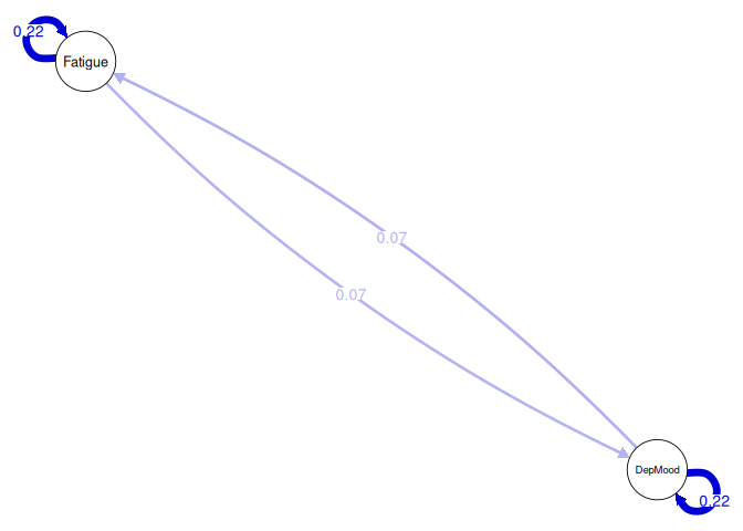
Interpretation:

• Bidirectional Influences: The network indicates that fatigue at time$t$ predicts increased depressed mood at time$t+1$, and vice versa, it suggests a reciprocal relationship where each variable influences the other over time.

• Self-Reinforcing Effects: The relative large autoregressive coefficients imply that a variable tends to maintain its state over time. For instance, if an individual experiences fatigue at time$t$, a positive autoregressive effect would suggest they are likely to experience fatigue at time$t+1$ as well.

Contemporaneous Networks

Beyond temporal dynamics, GVAR models also assess contemporaneous networks, which capture the relationships between variables within the same time point, after accounting for temporal effects. This is achieved by modeling the correlations among residuals (e.g.,${ϵ}_{y,t,i}$,${ϵ}_{z,t,i}$). Therefore, this network is a undirected network.

Unlike partial correlation networks in cross-sectional analysis (we have learned in the last chaptor), contemporaneous networks control for temporal dependencies, providing a clearer picture of instantaneous associations between variables.

# Plot the contemporaneous network
plot(model_mlVAR,          # The mlVAR model object containing the estimated networks
     type = "contemporaneous",    # Specify that we want to plot the contemporaneous network
     nonsig = "hide",      # Hide non-significant edges in the plot
     layout = "circle",    # Arrange nodes in a circular layout
     theme = "colorblind", # Apply a colorblind-friendly theme
     edge.labels = TRUE)   # Display edge labels indicating the strength of connections

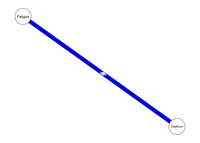
Interpretation:

• Simultaneous Experiences: A significant contemporaneous association between fatigue and depressed mood suggests that when an individual feels fatigued, they are also likely to feel depressed at the same time point, even after accounting for prior states of these variables.

fixed effect within a “hypothetical average person

In Graphic VAR, both temporal and contemporaneous networks often represent fixed effects —that is, they capture average within-person relationships across all individuals, describing a “hypothetical average person”. While there can be random effects for some or all parameters (e.g., random slopes), these are typically not displayed directly in the graphical network. Instead, the network plots reflect the central trend of how variables are interrelated within persons.

The temporal network illustrates how a typical person’s variables predict one another over time. Conversely, the contemporaneous network depicts how a typical person’s variables co-occur at the same time, beyond lagged influences.

Multilevel Graphical Vector Autoregression (mlVAR)

In previous discussions, we’ve explored how Vector Autoregression (VAR) models can be extended to Graphical VAR (GVAR) to analyze the dynamic interplay between multiple psychological variables over time. Building upon this, Multilevel Graphical Vector Autoregression (mlVAR) further incorporates the hierarchical structure of data, allowing for the examination of both within-person (intra-individual) and between-person (inter-individual) effects.

In the MLM section, we learned about the L1 and L2 predictors. When analyzing longitudinal data, the observed values of variables are L1 predictors; therefore, it can encompass both within-person fluctuations and stable between-person differences. To disentangle these components, we decompose each predictor using Centering Within Cluster(CWC) into:

• Within-Person (Intra-Individual) Component: Represents the deviation of an individual’s score at a specific time point from their own mean score across all time points.

• Between-Person (Inter-Individual) Component: Represents the individual’s mean score across all time points, reflecting stable traits or characteristics.

It can be written as:

$$ \begin{aligned} y_{t-1,i} &= \bar{y}i + \tilde{y}{t-1,i} \ z_{t-1,i} &= \bar{z}i + \tilde{z}{t-1,i} \end{aligned} $$

Where:

• ${\overline{y}}_i,{\overline{z}}_i$: Person-specific means (between-person components).
• $\tilde{y}{t-1,i}, \tilde{z}{t-1,i}$: Within-person centered values, calculated as the deviation of one time points from the person-specific mean.

By centering each person’s measurements around their own mean (CWC), we isolate intra-individual fluctuations. Including person-level means as separate predictors in the model reflects stable inter-individual differences.

Between-Person Network

Beyond temporal and contemporaneous within-person networks, mlVAR can estimate a between-person network based on individuals’ average scores on each variable across the entire time.

In our example, we could use the following code:

# Plot the between-person network
plot(model_mlVAR,          # The mlVAR model object containing the estimated networks
     type = "between",    # Specify that we want to plot the between-person network
     nonsig = "hide",      # Hide non-significant edges in the plot
     layout = "circle",    # Arrange nodes in a circular layout
     theme = "colorblind", # Apply a colorblind-friendly theme
     edge.labels = TRUE)   # Display edge labels indicating the strength of connections

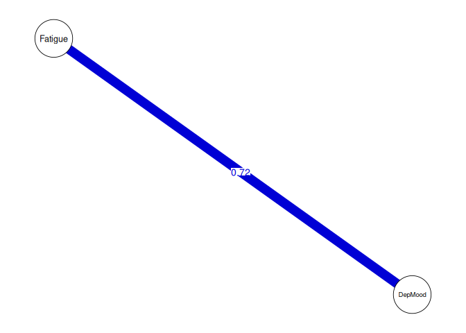
Interpretation:

• Between-Person Network: A significant edge between the mean levels of Fatigue and DepMood indicates that individuals who, on average, report higher levels of fatigue tend to, on average, report higher levels of depressed mood compared to others.

Comparison three Networks

• Temporal Networks: Depict how one variable predicts another (including itself) in the next measurement occasion, indicating directional influences over time.

• Contemporaneous Networks: Show relationships between variables within the same measurement occasion, after controlling for temporal effects.

• Between-Person Networks: Reflect associations between individuals’ average levels of variables across the entire study period, highlighting stable differences between individuals.

By examining all three in tandem, we gain a comprehensive understanding of psychological dynamics—from how symptoms or states evolve within individuals to how individuals differ between themselves on average.

Challenges in Estimating Parameter Covariances

Like we learned in the multilevel modeling (MLM) section, there can be covariances between random intercepts and random slopes. In multilevel Vector Autoregression (mlVAR), the situation becomes more complex because the model can include multiple random effects for each variable and its interactions over time.

For instance, in a bivariate mlVAR (with Depressed Mood and Fatigue), we typically estimate:

• Two person-specific intercepts (one for Depressed Mood, one for Fatigue) contributing to the temporal network.
• Two autoregressive slopes (how Depressed Mood predicts itself over time, how Fatigue predicts itself over time).
• Two cross-lagged slopes (how Depressed Mood predicts Fatigue at the next time point, and vice versa).
• Two random residuals (one for each variable) which contribute to the contemporaneous network (capturing within-time-point fluctuations after controlling for lagged effects).

Hence, we can have eight random effects in total, leading to many possible covariances in mlVAR. Accurately estimating these covariances is critical for unraveling how Depressed Mood and Fatigue interact and evolve within individuals over time.

When we account for covariances among random effects, it allows researchers to:

• Understand Interdependencies : A strong random slope covariance between Depressed Mood’s autoregressive effect and its cross-lagged influence on Fatigue could indicate that participants who show highly persistent Depressed Mood over time are also more prone to having their mood strongly predict future Fatigue. Another scenario might be that a negative covariance between Fatigue’s autoregressive random slope and its cross-lagged effect on Depressed Mood means that for individuals who show less stable Fatigue over time, there may be a weaker tendency for Fatigue to escalate subsequent Depressed Mood.

• Capture Individual Differences: Some individuals may exhibit high baseline (intercept) Depressed Mood and also high baseline Fatigue, with their intercepts being positively correlated. For them, Depressed Mood remains consistently elevated, and Fatigue often starts at a similarly high level. Meanwhile, other people might have lower baseline Depressed Mood but a stronger cross-lagged effect on Fatigue, suggesting that while they start off with less depressive mood on average, whenever they do experience Depressed Mood, it strongly predicts higher Fatigue at the next time point.

In each of these examples (it could have more), covariances among random effects reveal how the temporal or contemporaneous dynamics between Depressed Mood and Fatigue can vary considerably across individuals. Such insights are key to personalized approaches in both research and clinical practice, as they highlight the specific patterns through which variables reinforce or alleviate each other over time.

However, as the number of variables in an mlVAR model increases, the complexity of estimating parameter covariances grows exponentially. This is due to the need to integrate over high-dimensional distributions of parameters, which becomes computationally intensive and sometimes infeasible for models with many variables.

Estimation Strategies

To address these challenges, two primary estimation strategies are employed:

1. Correlated Estimation:

In correlated estimation, the model accounts for covariances between random effects by estimating a subset of these covariances. This method involves integrating over a high-dimensional parameter distribution to capture potential interdependencies among random effects.

However, in Correlated Estimation, not all covariances between random effects are estimated. Specifically, only the covariances among random effects that influence the same dependent variable are considered. This approach is adopted to manage computational complexity and to focus on the most relevant interdependencies.

In our example, the random effects ${\beta }_{01,i}$(person-specific intercept for Depressed Mood), ${\beta }_{11,i}$(autoregressive effect of Depressed Mood), and ${\beta }_{12,i}$(cross-lagged effect from Fatigue to Depressed Mood) all pertain to the variable Depressed Mood. Therefore, the covariances among these random effects are estimated. This allows us to understand how individual differences in baseline levels, stability over time, and the influence of Fatigue on subsequent Depressed Mood are interrelated.

Even only in this way, correlated estimation is typically practical for models with a smaller number of variables due to computational limitations. Computationally demanding and typically feasible only for models with up to six variables. Beyond this, the estimation process may become impractical due to the high computational burden.

2. Orthogonal Estimation:

Orthogonal estimation simplifies the model by assuming that random effects are uncorrelated, effectively setting covariances between them to zero. This assumption reduces the complexity of the model and the computational resources required for estimation. By not estimating covariances between random effects, orthogonal estimation reduces the number of parameters and the computational burden, making it feasible to estimate models with a larger number of variables (e.g., up to 20 nodes). It’s important to note that while the covariances between random effects are fixed at zero, the variance of each random effect is still estimated.

However, Assuming that random effects are uncorrelated may overlook meaningful interdependencies. This simplification can lead to a less accurate representation of the underlying dynamics between variables. Neglecting covariances between random effects might result in biased parameter estimates, potentially affecting the validity of the model’s conclusions.

Practical Considerations

When choosing between correlated and orthogonal estimation strategies, researchers should consider the following factors:

• Model Complexity: For models with a smaller number of variables, correlated estimation is feasible and can provide valuable insights into the relationships between random effects.

• Computational Resources: Orthogonal estimation is more suitable for larger models due to its reduced computational demands.

• Research Objectives: If understanding the interdependencies between random effects is crucial to the research question, correlated estimation may be preferred despite its computational challenges. Conversely, if the primary goal is to estimate fixed effects only in a large model, orthogonal estimation might be a practical alternative.

Visualizing Estimation Strategies

To enhance understanding of which covariances between random effects are estimated under different estimation strategies, we present a heatmap of the covariance matrix estimation.

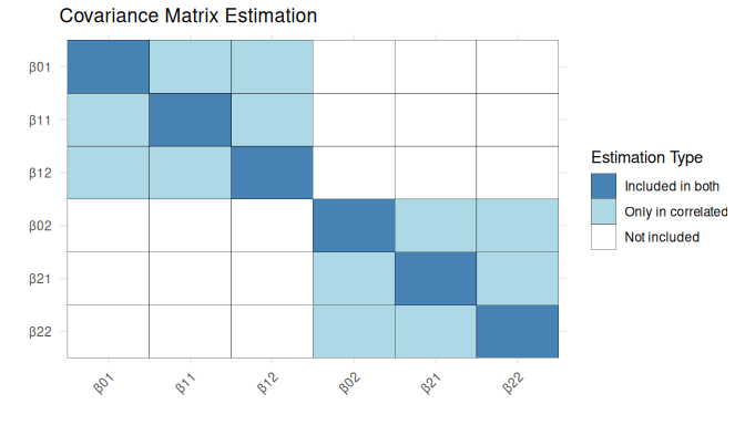
This visualization categorizes parameter covariances into three groups:

• Included in both estimation strategies (dark blue): These covariances are always estimated, regardless of whether Correlated Estimation or Orthogonal Estimation is used.
• Only in Correlated Estimation (light blue): These covariances are estimated only when using Correlated Estimation. In Orthogonal Estimation, they are fixed at zero.
• Not included (white): These covariances are never estimated in either approach.

By interpreting this figure, you can see that only covariances between random effects that influence the same dependent variable (Depressed Mood or Fatigue) are estimated under Correlated Estimation, while cross-variable covariances are not included. This reinforces the conceptual discussion before.

Assumptions of mlVAR

Stationarity

A fundamental assumption in mlVAR modeling is stationarity. This assumption implies that the statistical properties of the time series—such as mean, variance, and autocorrelation—remain constant over time. Stationarity is more plausible when data is collected over short time spans; however, for longer durations, this assumption may not hold due to potential underlying trends or evolving dynamics.

This assumption is important because mlVAR models estimate parameters like autoregressive effects (e.g., how Depressed Mood at one time point predicts itself at the next) and cross-lagged effects (e.g., how Fatigue at one time point predicts Depressed Mood at the next) as constant over the observed period. If the time series data are non-stationary, these estimated effects may not remain consistent over time, leading to potential biases and inaccuracies in the model’s conclusions. For instance, if there is an underlying trend causing Depressed Mood to increase over time, the model might misattribute this trend to the relationship between variables, rather than recognizing it as an external time influence.

Types of Non-Stationarity

Non-stationarity in time series data can manifest in two primary forms: Time Trends and Unit Root Processes.

1. Time Trends refer to systematic, deterministic changes in a time series over time, which can be either linear or nonlinear. These trends indicate that the mean of the series is changing, leading to non-stationarity.

Consider a scenario where individuals report their Depressed Mood scores over several months. If there’s a consistent increase in these scores, it suggests a linear upward trend, indicating that the average level of Depressed Mood is rising over time. This violates the stationarity assumption, as the series exhibits predictable patterns that evolve. As a result, the estimated autoregressive effects in mlVAR may become biased. The increasing trend may inflate the estimated influence of past Depressed Mood on future Depressed Mood, leading to misinterpretation of the true within-person dynamics.

2. A unit root process is a stochastic form of non-stationarity where a time series exhibits extremely high autocorrelation, meaning that its values strongly depend on previous observations. In mathematical terms, the standardized autoregressive coefficient is equal to 1, which causes the series to behave like a random walk.

In such a process, changes in the variable accumulate over time instead of reverting to a stable long-term mean. As a result, any shock or disturbance in the system can have permanent effects, making the series unpredictable and highly dependent on its historical values.

Imagine tracking daily Fatigue levels in a sample of individuals. Suppose there is a sudden increase in fatigue due to an external event (e.g., a stressful life event or illness) in the future. If the fatigue data follows a unit root process, this increase does not dissipate over time but rather persists, meaning that future fatigue levels is unpredictable.

Detecting Time Trends

One of the most effective methods for detecting Time Trends in time series data is visual inspection. By plotting the data over time, researchers can identify key indicators of non-stationarity, such as trends, shifts in variance.

Therefore, we need to create a simple time-series plot with time on the x-axis and the variable of interest on the y-axis. Suppose we plot variable DepMood, To inspect non-stationarity in the DepMood variable, we use a LOESS (Locally Estimated Scatterplot Smoothing) curve to visualize potential trends over time. LOESS is a flexible smoothing method that can fit any nonlinear relationship in the data by adjusting to local patterns without assuming a specific trend.

# Load ggplot2 for visualization
library(ggplot2)

# Plot DepMood over time using LOESS smoothing

ggplot(data, 
       aes(x = measurement_date, y = DepMood)) +  # Set x-axis as time and y-axis as DepMood levels
  geom_smooth(method = "loess", se = TRUE, color = "blue") + # Add LOESS smoothing with confidence interval 
  xlab(" ") +  # Remove x-axis label for cleaner visualization
  ylab(" ")  # Remove y-axis label for cleaner visualization

## `geom_smooth()` using formula = 'y ~ x'

## Warning: Removed 2134 rows containing non-finite outside the scale range (`stat_smooth()`).

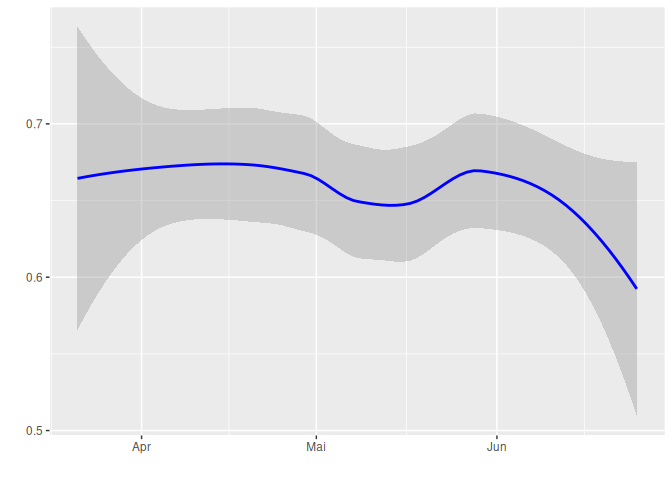
The plot below shows Depression mood over time, with a LOESS smoothing line and confidence intervals (shaded area). The trend appears to decline slightly over time, but the decrease is not severe. Since there is no strong upward or downward trend, we consider the data to be non time Trends.

In addition to visual inspection, statistical techniques can be employed to detect time trends in time series data. One effective method is the use of MLM like we leanred before. By incorporating time as a predictor, MLM can effectively identify and quantify time trends within the data.

For example, To assess whether Depressed Mood scores change over time, an MLM can be specified with (measurement)time as a predictor and individual participants as random effects.

# Load required packages
library(lme4)

## Loading required package: Matrix

library(lmerTest)  # For p-values in MLM

## 
## Attaching package: 'lmerTest'

## The following object is masked from 'package:lme4':
## 
##     lmer

## The following object is masked from 'package:stats':
## 
##     step

# Fit the Linear Mixed Model (LMM)
MLM_model <- lmer(DepMood  ~ measurement + (measurement | sub_id), data = data)

# View model summary
summary(MLM_model)

## Linear mixed model fit by REML. t-tests use Satterthwaite's method ['lmerModLmerTest']
## Formula: DepMood ~ measurement + (measurement | sub_id)
##    Data: data
## 
## REML criterion at convergence: 6890.4
## 
## Scaled residuals: 
##     Min      1Q  Median      3Q     Max 
## -3.9555 -0.4505 -0.0551  0.3630  4.9544 
## 
## Random effects:
##  Groups   Name        Variance  Std.Dev. Corr 
##  sub_id   (Intercept) 0.4009793 0.63323       
##           measurement 0.0004127 0.02032  -0.36
##  Residual             0.1661040 0.40756       
## Number of obs: 5390, groups:  sub_id, 228
## 
## Fixed effects:
##               Estimate Std. Error         df t value Pr(>|t|)    
## (Intercept)   0.692848   0.044108 227.423168  15.708   <2e-16 ***
## measurement  -0.001679   0.001515 221.782557  -1.108    0.269    
## ---
## Signif. codes:  0 '***' 0.001 '**' 0.01 '*' 0.05 '.' 0.1 ' ' 1
## 
## Correlation of Fixed Effects:
##             (Intr)
## measurement -0.433

A non-significant time effect would indicate there is no systematic (linear) trend in Depressed Mood over the observed period.

Addressing Time Trends

If a time trend is detected, it’s essential to adjust the data to meet the stationarity assumption required for many time series analyses. One common approach is detrending, which involves removing the identified trend from the data.

1. Fit a Regression Model: Regress the variable of interest (e.g., Depressed Mood) on time to capture the underlying trend.

Ideally, we should account for individual differences in time trends by employing a MLM, which allows for random slopes and intercepts, thereby modeling each person’s unique time trend over time. However, in practice, to simplify the analysis, it’s common to remove only the average effect of the time trend. This can be achieved by fitting a simple linear regression model with time as the predictor, effectively capturing and removing the overall trend from the data. This approach assumes that individual deviations from the average trend are negligible or that the primary interest lies in the fixed effect.

2. Extract Residuals: The residuals from this regression represent the variation in the data after accounting for the time trend.

3. Analyze Residuals: These residuals constitute the detrended series, which can now be analyzed under the assumption of stationarity.

The code can be written as:

# Fit a linear regression model (Depressed Mood ~ Time)
lm_model <- lm(DepMood ~ measurement, data = data)

residuals <- residuals(lm_model)

Note: Researcher recommend always detrending linear trends before estimating networks to prevent spurious associations.

Equidistant Measurements

In mlVAR, another fundamental assumption is that measurements are taken at equidistant time intervals. This means that the time difference between any two consecutive assessment points is equal, ensuring that the temporal dynamics are consistently captured across the study period.

When the assumption of equidistant measurements is violated, unequal time intervals can distort the estimation of temporal relationships between variables. Moreover, inconsistent time gaps may obscure the true nature of the relationships being studied, leading to incorrect conclusions.

However, in practical research settings, achieving perfectly equidistant measurements can be challenging due to various factors:

• Multiple Assessments Per Day: When participants provide multiple responses within a single day, the intervals between these assessments may vary. For instance, there might be shorter intervals between morning assessments and longer gaps overnight.

• Irregular Participation: Participants may miss certain assessments or respond at irregular times, leading to unequal time gaps between consecutive measurements.

Addressing Non-Equidistant Measurements in mlVAR:

To mitigate the issues arising from non-equidistant measurements, the mlVAR package offers specific arguments:

1. dayvar: This argument specifies the variable that indicates the assessment day. By including dayvar, the model ensures that the first measurement of a day is not regressed on the last measurement of the previous day, thereby preventing erroneous temporal connections across days.

2. beepvar: This optional argument indicates the assessment beep per day. When beepvar is provided, non-consecutive beeps are treated as missing, ensuring that only consecutive assessments within the same day are considered in the temporal modeling.

Im summary, if the data collection schedule is consistent and does not include irregular intervals, specifying only the beepvar argument is sufficient to account for the measurement structure. However, if the data includes such irregularities, both dayvar and beepvar should be specified to accurately model the temporal dynamics.

Extracting Specific Networks from the mlVAR Model

In psychological research, we have learned from the last chapter that individual differences in network connectivity is crucial. For instance, in this study, the research want to test if a person with a highly interconnected affective network may experience more persistent or severe depressive episodes.

To investigate this question, we can extract specific networks from the mlVAR model using the getNet() function from the mlVAR package. This function allows researchers to obtain the estimated network structures—temporal, contemporaneous, or between-subjects—for further analysis.

For example, we can extract the temporal network as follows:

# Extract the temporal network
temp1 <- getNet(model_mlVAR, "temporal", subject = 1) # extract from the first person

## 'nonsig' argument set to: 'show'

temp2 <- getNet(model_mlVAR, "temporal", subject = 2) # extract from the second person

## 'nonsig' argument set to: 'show'

If we only want to the fixed effect instead of a special person, then we can easily delete the argument subject =.

Investigating Temporal Network Connectivity

Once the temporal network is extracted from the mlVAR model, we can assess its overall connectivity between variables. Instead of using Average Shortest Path (APL) which we have leaned from last part, in this study, the author used Network density (average absolute weight).

The density of a network is calculated as:

$$Density=\frac{1}{n}\sum _{i=1}^n|w_i|$$

Where:

• $n$ = Total number of edges in the network.
• $w_i$ = Weight of the$i$-th edge.

The code is:

mean(abs(temp1)) # calculate the network density for the fitst person's temporal network

## [1] 0.1305905

Comparison to Average Shortest Path

Below, we compare these two measures of network connectivity in terms of their strengths and limitations.

Advantages of Network Density (Compared to Average Shortest Path):

• Computational Simplicity: Unlike Average Shortest Path, which requires computing distances between all pairs of nodes, network density is based only on the sum of edge weights, making it much easier and faster to calculate.
• Considers Edge Weights: Unlike the Average Shortest Path (as we learned it, without considering edge weights), network density explicitly incorporates the strength of connections. This means that stronger connections contribute more to density than weaker ones, making it a more informative measure in weighted networks.

Disadvantages of Network Density (Compared to Average Shortest Path):

• Ignores Network Topology: Unlike Average Shortest Path, which captures how nodes are positioned relative to each other, network density does not consider whether connections are clustered or spread out.
• Misses Indirect Relationships: The Average Shortest Path accounts for indirect paths (i.e., connections that pass through multiple nodes), while network density only considers direct edges, potentially overlooking important structural dynamics in the network.
• Lack of Interpretability in Some Contexts: While a high density suggests strong connectivity, it does not indicate whether the network is efficiently structured or overly rigid, whereas Average Shortest Path provides insight into how easily activation or influence spreads between nodes.

When to Use Each Metric?

• Use Network Density when the goal is to get a quick and simple measure of overall connectivity and when considering edge strength is important.
• Use Average Shortest Path when interested in how efficiently nodes communicate or how activation spreads through both direct and indirect connections.

Advanced Topic: Time-Varying Vector Autoregressive (TV-VAR) Models

In traditional VAR, a key assumption is stationarity. However, in many psychological and behavioral studies, this assumption may be violated as the underlying dynamics of the system evolve. To address this, Time-Varying VAR (TV-VAR) models have been developed, allowing parameters to change over time.

When the assumption of stationarity is violated, instead of assuming a static network, researchers can estimate network models at each time point to observe how connections between variables fluctuate.

Concept of “Data-Borrowing”

A significant challenge in TV-VAR modeling is the limited data available at each time point. To mitigate this:

• Single Observation Per Time Point: Typically, there’s only one observation per time point, making it difficult to estimate parameters reliably.

• Borrowing Data from Nearby Time Points: By assuming that observations close in time are generated by similar processes—a concept known as local stationarity—data from adjacent time points can be utilized to enhance estimation accuracy.

To effectively borrow data from nearby time points:

• Assumption of Local Stationarity: It’s presumed that time points close to each other are influenced by similar underlying mechanisms.

• Proximity-Based Weighting: Data from nearer time points are assigned higher weights, reflecting the belief that they share more similar dynamics compared to more distant observations.

Bandwidth in TV-VAR Models

A crucial parameter in TV-VAR modeling is the bandwidth, which determines the range of time points considered when estimating parameters at a specific time:

• Definition: Bandwidth controls the width of the window around each time point, dictating how many neighboring observations are included in the estimation process.

• Impact: A larger bandwidth incorporates more data, potentially smoothing over rapid changes, while a smaller bandwidth allows for capturing more abrupt transitions but may result in noisier estimates.

For a comprehensive understanding of TV-VAR models and their estimation methods, refer to the tutorial by Haslbeck et al. (2021), which provides an in-depth discussion on this topic.

Example

To illustrate the application of TV-VAR models, consider the following example where we analyze the time-varying relationship between Fatigue and Depressed Mood.

# Load the mgm package
library(mgm)

# Define model parameters
variables <- c("Fatigue", "DepMood")  # Variables to include in the model
lags <- 1  # Number of lags to include in the model
bandwidth <- 1  # Bandwidth parameter for kernel smoothing; adjust based on data characteristics

# Remove rows with missing values from the dataset
data_clean <- na.omit(data)

# Estimate the time-varying VAR model
tvvar_model <- tvmvar(
  data = data_clean[, variables],      # Use the cleaned data with selected variables
  type = rep("g", length(variables)),  # Assume variables are continuous ("g" denotes Gaussian)
  level = rep(1, length(variables)),   # For continuous variables, set level to 1
  lags = lags,                         # Specify the number of lags
  estpoints = seq(0, 1, length = 100), # Proportional locations of estimation points
  bandwidth = bandwidth,                # Bandwidth parameter for kernel smoothing
  pbar = F
)

## Note that the sign of parameter estimates is stored separately; see ?tvmvar

# Extract parameter estimates
parameter_values <- tvvar_model$wadj[2, 1, 1, ] # here we only extact one effect as example

# Plot the parameter estimates over time
plot(parameter_values, type = "l", ylim = c(0, 0.4),
     lwd = 2, ylab = "Parameter Value", xlab = "Estimation Points",
     main = "Time-varying cross lagged effect of Fatigue on Depressed Mood")

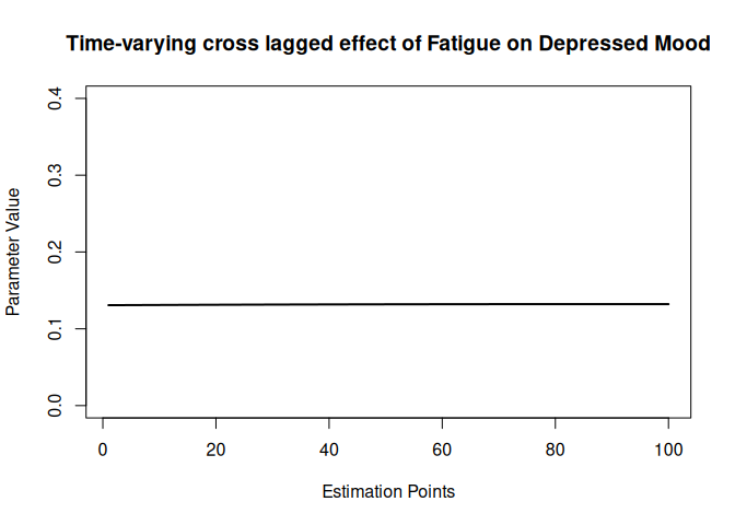
The resulting plot displays the time-varying effect of Fatigue on Depressed Mood with a lag of 1. The x-axis represents the estimation points, which correspond to specific time intervals in the data. The y-axis indicates the estimated parameter values, reflecting the strength of the relationship between the two variables at each time point.

Here we observed a nearly horizontal line, indicating that the cross lagged effect of Fatigue on Depressed Mood remains relatively constant throughout the observed period. This finding underscores the stationarity assumption before opting for time-varying models.

References

Cohen, J. (1988). Statistical power analysis for the Behavioral Sciences. Routledge. Hamaker, E. L. (2012).Why researchers should think” within-person”: A paradigmatic rationale.

Epskamp, S. (2020). Psychometric network models from time-series and panel data. Psychometrika, 85(1), 206-231.

Haslbeck, J. M., Bringmann, L. F., & Waldorp, L. J. (2021). A tutorial on estimating time-varying vector autoregressive models. Multivariate behavioral research, 56(1), 120-149.

Molenaar, P. C. (2004). A manifesto on psychology as idiographic science: Bringing the person back into scientific psychology, this time forever. Measurement, 2(4), 201-218.

Lunansky, G., Hoekstra, R. H., & Blanken, T. F. (2023). Disentangling the Role of Affect in the Evolution of Depressive Complaints Using Complex Dynamical Networks. Collabra: Psychology, 9(1).