](/media/header/sunny_coastal.jpg)
The student's guide to independence in R
Contents
- 1. Introduction
- 2. How do I get started?
- 3. Common analysis steps
- 3.1. I. Reading raw data
- 3.1.1. An aside about file paths
- 3.2. II. Cleaning up and preprocessing raw data
- 3.3. III. Aggregate raw data
- 3.4. IV. Descriptive analysis and plots
- 3.4.1. Descriptive stastics: Getting a sense of your data
- 3.4.2. Confidence intervals
- 3.4.3. Data visualisation magic
- 3.4.3.1. Boxplots
- 3.4.3.2. Adding titles and labels
- 3.4.3.3. Spaghetti plots
- 3.4.3.4. Fancy Barplots
- 3.4.3.5. Visualizing correlations with scatter plots
- 3.5. V. Inferential analysis
- 3.5.1. Normality assumption
- 3.5.2. Homogeneity of variance assumption
- 3.5.3. Correlation
- 3.5.4. Regression
- 3.5.5. t-test
- 3.5.6. One-way ANOVA
- 3.5.7. Repeated measures ANOVA
- 3.5.8. Mixed designs (within/between factors)
- 3.1. I. Reading raw data
- 4. General notes on
R|
Introduction
Dear students,
This tutorial was developed for thesis students at LISCO lab (Lifespan Brain and Cognitive Development lab, Goethe-University Frankfurt am Main) and may also be useful in other contexts.
In this tutorial, I - Dr. Sophie Nolden - will provide some tips that are meant to help you to use R independently. This implies that you find own solutions for your analyses, with operations and functions that are new to you. If you are students at Goethe-University, most of you have already worked with R in the Expra or other courses, and things may have seemed very clear to you back then. However, when you have to create your own analysis script from scratch, you may sometimes be a little lost. I thus summarized a few key points that can help you to find your way in the jungle!
Please make sure that you always try to figure out the solution yourself first. If you are stuck, ask your peers (or your supervisor if your peers cannot help you), and make sure that you provide all the information needed to understand both your question and your first approach to solve the problem.
Enjoy reading!
You should be familiar with some basics in R before you continue, have a look at these notes, for example.
If you need more input, I suggest to work with an online tutorial of your choice. For example, check out these three (1, 2, 3) suggestions on first steps in R.
You may also want to checkout the documentation on R Markdown.
The Department of Psychological Methodology at the Psychology Faculty of Goethe-University has also created pandaR - the very site you are reading this tutorial on. pandaR was first created in order to present projects to deepen your skills in R and to experiment around with the contents of the module PsyBSc2 that aims to teach students the statistical basics in R. Since then, the team has worked on uploading detailed tutorials on various statistical measures and applications. Have a look at the page Lehre where you can find an overview of all the topics that are dealt with in the statistics lectures.
On pandaR you’ll find a general introduction to R that offers a very detailed explanation of the most important functions of the software (in German). Feel free to take a look, if you are new to R!
You should now know the following concepts (please test yourselves):
- What is a data frame? How is it different from a matrix?
- How can I access certain data points in a data frame? How can I select certain rows or columns?
- Which classes of data are there?
- What is a function and how is a function different from a script?
- What is a boolean expression?
- Why are there different packages? How can I install packages?
How do I get started?
Before you write your first line of R code, make sure that you know exactly what you would like to do and how you want to do it.
Here are some examples for very general questions: Do you want to calculate an average? Do you want to calculate a t-test or rather a correlation? What are your independent and dependent variables?
Once your general approach is clear, ask yourself more specific questions such as: In which columns of my data frame do I find my independent or dependent variables? Do I want to correct for outliers? Which lines should be deleted if I want to exclude practice blocks?
Just imagine your data frame was a table on a physical sheet of paper and your only tools were a pen and a simple calculator. What would be your analysis steps?
Very often, students tell me that they do not know how to handle R, but once I start asking questions about their analysis plan, I realize that they actually do not know what they want to do! So make sure that every single step of your analysis is clear to you. I suggest to write down your analysis steps into your script (as comments). Once you are done and your concept makes sense to you, you can fill it up with actual code. This way, you have already made sure that your documentation is well done, since there should be a balance of 50:50 between comments and code.
Generally speaking, your script should be structured like this:
- Start your script with a title, your name, and the current date. If your script is based on an older script, provide this information as well.
- Clean up your global environment.
rm(list = ls())
- Continue with your parameters. These are values that you may eventually want to change and that you do not want to search for in every single line of your script. For example, you write your data path here, or you define the different age groups that you have tested. Just make sure you write your script in such a way that you can use it at multiple occasions (which may become relevant for your thesis).
- Continue with your actual analysis. Provide some structure and comment on everything you do. Documentation is important so that the script is understandable for others, both your collaborators and your future self.
Where can I get help?
After you gained some basic knowledge in R, you should definitely not expect to sit down in front of your computer and then, magically, your fingers just type down all the code. It is a matter of constant improvement, and you will have to learn how to use new functions all the time!
It is normal to look up how to do certain things, even if you have dealt with a similar problem before.
Here are four main sources of help for your script:
- Recycle elements from previous scripts. Create functions for recurring problems. This is actually quite useful because you have already figured it out once before. Remember to always provide comments on what you are doing in the script, in order to be able to recycle stuff in the future.
- Use a search engine of your choice and look up your question in the internet. The community is huge and usually very friendly, and chances are quite high that somebody else has encountered your problem before. (You can also post questions yourself if nobody has asked your questions before, but this will most likely not be the case.) Search in English. I like pages such as
stackoverflowandgithubfor helpful discussions. It will take some time until you know how to ask your questions properly. Your first search term should of course be “R”. Use key words fromRand psychology, such as “data frame”, “columns”, “outlier”… If you put too many terms into the search window, you will probably get a lot of results that are not related to your question, so try to be precise. When you realize that the answers you get are rather remote from what you actually want, change your search terms. - Use the help function in
R. This requires some practice and may not always help you when you are new to it. I find it most useful for the list of input arguments and the examples provided in the end. - As mentioned before, you will find many detailed tutorials on specific statistical topics on pandaR.
This is how you deal with the help function.
help(<function>)
?<function>
help.start()
Use apropos(<topic>) in case you do not know the name of a specific function.
apropos('anova')
## [1] "anova"            "manova"           "power.anova.test" "stat.anova"
## [5] "summary.manova"
Use example(<topic>) if you want to see an example.
You can copy the code for any boxplot example from your console and run it or you can press enter to get a new example. Type stop() when you’ve had enough and you can go back to running new code.
Common analysis steps
All analyses are of course different, but there are some common analysis steps that we encounter most of the time:
- Reading raw data
- Cleaning up and preprocessing raw data
- Aggregating raw data
- Descriptive analysis and plots
- Inferential analysis
We will go through them step by step.
I. Reading raw data
Getting error messages in R can be frustrating at the beginning. However, it is quite normal, and you will learn to read the error messages in a way that they can guide you to the solution. Not handling your raw data properly, on the other hand, can lead to REAL PROBLEMS!!!
You have to be super careful with your raw data. Store it at multiple sites on different drives. And NEVER, really NEVER EVER, write into your raw data directory. This is why we call our raw data directory sometimes “Holy Folder”, and it must NEVER be touched other than for reading the data so that you can never accidentally overwrite it.
That is why we need an “in_path” and an “out_path”, one directory to read from, one to write into. Create a directory with all participants’ raw data. If you already know that you want to exclude a participant for whatever reason, you can already omit the respective file at this stage. Create a directory called “Analyses” or something similar. Always choose meaningful names and avoid spaces or special characters.
# Define in_path.
in_path <- "/home/soph/Documents/thesis/Holy_Folder/"
# Define out_path.
out_path <- "/home/soph/Documents/thesis/Analyses/"
in_path
## [1] "/home/soph/Documents/thesis/Holy_Folder/"
out_path
## [1] "/home/soph/Documents/thesis/Analyses/"
It is very common that there are errors in your paths. In order to avoid typos, I suggest that you browse to your directory and then copy the path from there (e.g., from your browser header, or by selecting the properties of a file in that directory). This can be especially helpful for long and complicated paths. If you use Windows, you may need to change the slashes. R only recognizes forward slashes, therefore you have to replace all backwardslashes. Try Ctrl + F; in the search bar you can “find” all backslashes and “replace” them with forward slashes by clicking on “All” on the very right of the bar.
Make sure that you do not forget the " “.
And, last but not least, and that is very often overlooked by beginners: Do not forget the last slash in the end! ;-)
You can also set your working directory in R via “Session” -> “Set Working Directory” (to your out_path).
I recommend to never use spaces or special characters in your path. It may be worthwhile renaming your directories. The same is true for all objects/column names/characters you create in R. It is not impossible to handle spaces in R, but it is definitely more troublesome.
Remember that your paths should be defined at the beginning of your file.
An aside about file paths
As you begin using R in more of your projects, some of which may involve collaboration, you may begin to notice that dealing with paths and working directories can get, well, pesky. An example: your colleague Bailey sends you a folder with their data and analysis scripts. In the script, they begin with setting the working directory using:
setwd("C/Users/bailey/Documents/projectA/analysis/")
Or at various points in the file, they load data using:
load("C:/Users/bailey/Documents/projectA/analysis/somefolder/blahblah.rda")
It’s easy to see how the specificity of file paths can quickly get annoying and make the script fragile. You are not Bailey, so you will have to change all of the paths in the files for the script to work again. And what if you were working on a script but then you get a new computer? What if you forgot one tiny “/” and now you want to set your computer on fire? And so on and so on.
A package that offers answers to these issues is the here() package. Combined with a logical folder structure, here() can improve the flexibility of your scripts so that neither you nor your collaborators will have to rename another file path again. Anywhere you would use “C:/filepath/blahblah”, you can replace with here(). You can check out a straightforward guide to using it here (no pun intended).
Let’s have a look at a few cases that you may run into
- We very often read data from
.csvfiles. There are specific functions for reading.csvfiles that you can use. I personally prefer the functionfreadbecause it can handle various data types quite easily.
This is how you can read all your participants’ data files into one data frame at once:
library(data.table) # fread is part of the library "data.table".

filenames <- list.files(inPath, pattern="*.csv", full.names=TRUE) # Create a list of your data files.

myData <- rbindlist(lapply(filenames,fread),fill=TRUE) # Read in your data files and concatenate them to one big data frame.
- Sometimes, you may need to open data files saved with
SPSS.SPSSis a commercial software and not everybody may have the license installed, so it can be quite tricky to open these kinds of files. I suggest to use the packagehavenfor this matter.
library(haven) # This library is useful to deal with SPSS files.

SPSSfile <- "myOtherData.sav" # Define the name of your SPSS file.

myOtherData <- read_sav(paste(inPath, SPSSfile, sep = "")) # Read in SPSS data. Note how I used "paste" to concatenate two character values (your path name and your file name).``
- If you tested multiple groups (e.g., children, young adults, and older adults), you may want to organize their data in different folders. In this case, I recommend to loop through these folders and add up all files into one single data frame. Just provide a vector of character values as “in_path”, with each character vector representing one path.
# Define in_path.
in_path <- c("/home/soph/Documents/thesis/Holy_Folder/Child/"
              , "/home/soph/Documents/thesis/Holy_Folder/YA/"
              , "/home/soph/Documents/thesis/Holy_Folder/Child/OA/")
Next, create an empty data frame with the same amount of columns and the same column name as in your actual raw data.
all_groups <- setNames(data.frame(matrix(ncol = 9, nrow = 0))
                       , c("participant", "group", "age", "sex", "handedness"
                       , "IV1", "IV2", "DV1", "DV2"))
Loop through the different directories and read the data from each directory one after another (e.g., into a data frame called “my_data”). Add it all to your empty data frame at the end of each iteration.
all_groups <- rbind(all_groups, my_data)
Tip 1 for using loops: Restrict the use of loops to a minimum, since R is not really fast dealing with loops (but it will do it eventually).
Tip 2 for using loops: Use a meaningful term for the value that changes at each iteration. “val” or “i” are not meaningful, but “i_group” or “i_participant” are. This will help you to keep track of what you are actually doing, especially in nested loops.
If you are interested in finding out more about loops and the (literally) endless possibilites that they offer, you can check out the tutorial on them on pandaR.
- In some cases, multiple files are generated per participant and you may want to merge the different files. For example, in a memory study, you have one file for a memory encoding session and one file for a memory retrieval session. It can be useful to have the two sessions organized as different columns and each line referring to a specific stimulus. In this case, check out a “merge” function (I like the one from the package “data.table”) in these cases.
Once your data are all in, you should take some time to check if all data looks as it is supposed to be. Are all subjects there? Is the number of lines as expected (this is very often the number of trials by the number of participants)? Are all conditions there? Is the number of trials for each condition correct?
For this purpose, use the table function. Have a look at your “global environment” as well where you can see the dimensions of your data frame.
If you still have questions about loading your data into R or if you’re still unsure on how the working directory works, have a look at the R crash course on pandaR, where all these topics are discussed in more detail.
II. Cleaning up and preprocessing raw data
Our raw data files are usually organized such that one line contains all information from one trial. However, there may be trials that we do not need, such as practice trials. Or there may be empty lines between blocks that we also do not need.
Let’s have a look at the following example:
# Let's create a little example data frame.
example1 <- setNames(data.frame(matrix(ncol = 5, nrow = 10))
                    , c("participant", "OS", "block_number", "DV", "IV"))
# Values in columns.
example1[1:5,1] <- 5
example1[6:10,1] <- 6
example1[,2] <- as.character("Windows")
example1[,3] <-c(NA,1,1,2,2,NA,1,1,2,2)
example1[,4] <- c(.5,.6,.7,.7,.8,.9,.9,.8,.5,.7)
example1[,5] <- c("B","A","B","B","A","B","B","A","B","A")
example1
##    participant      OS block_number  DV IV
## 1            5 Windows           NA 0.5  B
## 2            5 Windows            1 0.6  A
## 3            5 Windows            1 0.7  B
## 4            5 Windows            2 0.7  B
## 5            5 Windows            2 0.8  A
## 6            6 Windows           NA 0.9  B
## 7            6 Windows            1 0.9  B
## 8            6 Windows            1 0.8  A
## 9            6 Windows            2 0.5  B
## 10           6 Windows            2 0.7  A
Side note: if you want to learn more about creating data frames, have a look at our R crash course, starting from the block “Daten”.
The column “block_number” contains, well, the block number. Lines with NA are practice trials. We can remove them like this:
example1 <- example1[!is.na(example1$block_number),] # Check the different parts of this line. What do the "!" and "is.na" do? Also check out the position of the comma in the square brackets. Remember: Rows first, columns later on!
example1
##    participant      OS block_number  DV IV
## 2            5 Windows            1 0.6  A
## 3            5 Windows            1 0.7  B
## 4            5 Windows            2 0.7  B
## 5            5 Windows            2 0.8  A
## 7            6 Windows            1 0.9  B
## 8            6 Windows            1 0.8  A
## 9            6 Windows            2 0.5  B
## 10           6 Windows            2 0.7  A
We probably also want to remove the column “OS” because it is not very helpful here. You can select specific columns by index or name, and you can also delete specific columns.
The following three code chunks do the same thing:
example1_copy <- example1 # Let's create a copy of example1 so we can do the same stuff over and over again.
example1 <- example1[,c(1,3,4,5)] # Select certain columns by index. Check out the position of the comma.
example1
##    participant block_number  DV IV
## 2            5            1 0.6  A
## 3            5            1 0.7  B
## 4            5            2 0.7  B
## 5            5            2 0.8  A
## 7            6            1 0.9  B
## 8            6            1 0.8  A
## 9            6            2 0.5  B
## 10           6            2 0.7  A
example1 <- example1_copy # Back to our previous data frame.
example1 <- example1[,c("participant", "block_number", "IV", "DV")] # Select certain columns by name.
example1
##    participant block_number IV  DV
## 2            5            1  A 0.6
## 3            5            1  B 0.7
## 4            5            2  B 0.7
## 5            5            2  A 0.8
## 7            6            1  B 0.9
## 8            6            1  A 0.8
## 9            6            2  B 0.5
## 10           6            2  A 0.7
example1 <- example1_copy # Back to our previous data frame.
example1$OS <- NULL # Delete a single columns by its name.
example1
##    participant block_number  DV IV
## 2            5            1 0.6  A
## 3            5            1 0.7  B
## 4            5            2 0.7  B
## 5            5            2 0.8  A
## 7            6            1 0.9  B
## 8            6            1 0.8  A
## 9            6            2 0.5  B
## 10           6            2 0.7  A
Actually, this would also be a good moment to organize the order of your columns in a more useful way. I prefer to start with the participant number, the group, time of testing, personal information like age and gender, information on stimuli, independent variables, and dependent variables in the end.
In the example above, it could be nice to switch the position of the independent and dependent variable.
The following two code chunks do the same thing:
example1 <- example1_copy # Back to our previous data frame.
example1 <- example1[,c(1,3,5,4)] # Omit the second block and switch the two last blocks.
example1
##    participant block_number IV  DV
## 2            5            1  A 0.6
## 3            5            1  B 0.7
## 4            5            2  B 0.7
## 5            5            2  A 0.8
## 7            6            1  B 0.9
## 8            6            1  A 0.8
## 9            6            2  B 0.5
## 10           6            2  A 0.7
example1 <- example1_copy # Back to our previous data frame.
example1 <- example1[,c("participant", "block_number", "IV", "DV")] # Or use the variable names.
example1
##    participant block_number IV  DV
## 2            5            1  A 0.6
## 3            5            1  B 0.7
## 4            5            2  B 0.7
## 5            5            2  A 0.8
## 7            6            1  B 0.9
## 8            6            1  A 0.8
## 9            6            2  B 0.5
## 10           6            2  A 0.7
Sometimes, you need to calculate new variables. Imagine the participants’ task was to indicate if a letter was a vowel or a consonant with a left or a right key press. Imagine also that the response mapping was counterbalanced, hence, half of the participants were supposed to respond to a vowel with a left key press and to a consonant with a right key press whereas the other half of the participants had the reversed mapping. Your software may have recorded whether the participants responded with a left or a right key press at a given trial, but not necessarily if participants wanted to indicate that they saw a vowel or a consonant, and if their response was correct. Let’s check out how we could create new variables in this case.
Let’s create another little example data frame.
# Let's create a little example data frame.
example2 <- setNames(data.frame(matrix(ncol = 4, nrow = 8))
                    , c("participant", "stimulus", "counterbalancing", "response"))
# Values in columns.
example2[1:4,1] <- 1
example2[5:8,1] <- 2
example2[,2] <- c("V","C","C","V","C","V","C","V")
example2[,3] <-c("vowel_left", "vowel_left", "vowel_left", "vowel_left", "cons_left", "cons_left", "cons_left","cons_left")
example2[,4] <- c("l", "r", "l", "l", "l", "l", "r", "r")
example2
##   participant stimulus counterbalancing response
## 1           1        V       vowel_left        l
## 2           1        C       vowel_left        r
## 3           1        C       vowel_left        l
## 4           1        V       vowel_left        l
## 5           2        C        cons_left        l
## 6           2        V        cons_left        l
## 7           2        C        cons_left        r
## 8           2        V        cons_left        r
Let’s first calculate a new variable that contains the meaning of the response.
example2$response_type <- "V" # As a default we put vowel.
example2$response_type[example2$counterbalancing == "vowel_left" & example2$response == "r"] <- "C" # If the participant is supposed to indicate consonants with the right response (belongs to the first counterbalancing group) and responded with the right key.
example2$response_type[example2$counterbalancing == "cons_left" & example2$response == "l"] <- "C" # If the participant is supposed to indicate consonants with the left response (belongs to the second counterbalancing group) and responded with the left key.
example2
##   participant stimulus counterbalancing response response_type
## 1           1        V       vowel_left        l             V
## 2           1        C       vowel_left        r             C
## 3           1        C       vowel_left        l             V
## 4           1        V       vowel_left        l             V
## 5           2        C        cons_left        l             C
## 6           2        V        cons_left        l             C
## 7           2        C        cons_left        r             V
## 8           2        V        cons_left        r             V
Let’s calculate accuracy as well: 0 = incorrect response, 1 = correct response.
example2$accuracy[(example2$stimulus == "V" & example2$response_type == "V") | (example2$stimulus == "C" & example2$response_type == "C")] <- 1 # Let's find the cases where stimulus and response_type match. Have a look at how I combined logical "and" and "or" and how I used brackets here.
example2$accuracy[is.na(example2$accuracy)] <- 0 # Now let us fill up with zeros for the incorrect responses.
example2
##   participant stimulus counterbalancing response response_type accuracy
## 1           1        V       vowel_left        l             V        1
## 2           1        C       vowel_left        r             C        1
## 3           1        C       vowel_left        l             V        0
## 4           1        V       vowel_left        l             V        1
## 5           2        C        cons_left        l             C        1
## 6           2        V        cons_left        l             C        0
## 7           2        C        cons_left        r             V        0
## 8           2        V        cons_left        r             V        1
Once again, check if all data are as they are supposed to be! The table() function helps you here.
If everything looks good, this would be a good moment to save your data frame to disk, e.g., in a .csv file.
III. Aggregate raw data
Aggregating means summarizing your data. For example, you may be interested in averaging all trials of each condition and each participant. For example, if you have two conditions, you may want to average all trials such that there are two averages per participant in the end, one for each condition.
Sometimes, we need to exclude outliers before we average raw data. For example, when you average response times, very slow responses may bias your averages strongly. You do not want to include these response times in your analysis. This is how you can proceed:
- Use the function “group_by” of
dplyrto group your data frame by participant. This could look like this:
my_data <- group_by(my_data, participant)
You may be disappointed: Your data frame looks as it has looked before. However, all consecutive commands will be executed within the trials belonging to the same participant. Later, use ungroup if you do not want grouping anymore.
- Create a new column that contains your z-transformed response times. There are plenty of ways to do the z-transform. I like the function
scale(). - Delete all rows that contain a z-value that exceeds your criterion (e.g., 3). You already know how to do this! Check out the “clean up raw data” section for inspiration!
In a similar way, you can also remove very fast responses, e.g. < 50 ms. In this case, you can work directly with the raw response times, no need for transforms!
Let us continue. I will provide an example data frame for you with one between IV, one within IV, and accuracy as DV:
example3 <- setNames(data.frame(matrix(ncol = 4, nrow = 12))
                    , c("participant", "IV1", "IV2", "accuracy"))
# Values in columns.
example3[1:6,1] <- 5
example3[7:12,1] <- 6
example3[,2] <- c('r','r','r','r','r','r','s','s','s','s','s','s')
example3[,3] <- c('B','A','A','B','A','B','A','B','A','A','B','B')
example3[,4] <- c(0,1,1,0,0,1,1,1,1,1,0,1)
example3
##    participant IV1 IV2 accuracy
## 1            5   r   B        0
## 2            5   r   A        1
## 3            5   r   A        1
## 4            5   r   B        0
## 5            5   r   A        0
## 6            5   r   B        1
## 7            6   s   A        1
## 8            6   s   B        1
## 9            6   s   A        1
## 10           6   s   A        1
## 11           6   s   B        0
## 12           6   s   B        1
When you create your script, you need to test it very carefully. Thus, when you work on the data aggregation, I strongly recommend to use an example data frame as the one above to try if everything works as you want it to work. Your raw data frame will very likely contain thousands of lines and chances are high that you would miss out on errors if you worked with the entire raw data frame.
You do not necessarily need to create a completely artificial example data frame. You can also select a limited amount of lines from your “real” raw data, e.g., you select two participants and for each participant 5 trials of all possible conditions. Just make sure that you think of all possible combinations of relevant variables when creating your example raw data frame.
Let us turn to the actual aggregation. I recommend the function “aggregate” from “stats”:
# Aggregate data (summarize over the within IV, separate for each participant).
agg_example3 <- aggregate(example3$accuracy # Which variable should be aggregated?
                    ,list(example3$IV1,example3$participant,example3$IV2) # How should we split up the new data frame?
                   ,mean) # What is our actual operation?
agg_example3
##   Group.1 Group.2 Group.3         x
## 1       r       5       A 0.6666667
## 2       s       6       A 1.0000000
## 3       r       5       B 0.3333333
## 4       s       6       B 0.6666667
The column names do not look especially fancy, so let us rename them.
# Create sensible column names.
colnames(agg_example3) <- c('IV1'
                        ,'participant'
                        ,'IV2'
                        ,'accuracy') #Name the columns with a vector containing the labels.
agg_example3
##   IV1 participant IV2  accuracy
## 1   r           5   A 0.6666667
## 2   s           6   A 1.0000000
## 3   r           5   B 0.3333333
## 4   s           6   B 0.6666667
We can now arrange the data frame the way we want, just as we did it with the raw data.
# Re-order columns.
agg_example3 <- agg_example3[,c(2,1,3,4)]

# Sort lines.
agg_example3 <- agg_example3[order(agg_example3$participant),]
agg_example3
##   participant IV1 IV2  accuracy
## 1           5   r   A 0.6666667
## 3           5   r   B 0.3333333
## 2           6   s   A 1.0000000
## 4           6   s   B 0.6666667
When the aggregation of your example data frame works correctly, turn to the real raw data. Once you’re done, check again if everything worked correctly. I suggest that you think of all possible cases/constellations and check if they worked for a few randomly selected subjects.
Again, the table() function is your friend here!
Once you have aggregated your raw data, you may still need to do a few adjustments to your data frame in order to get prepared for your further analyses.
One common dependent variable we use in memory research is the recognition probability (Pr) in recognition tests. This is the difference of hit rates and false alarm rates. Sometimes, we have different conditions during learning (e.g., expected or surprising objects) and thus, you end up with hit rates for expected and surprising objects. If your new objects do not allow you to separate between expected and surprising objects, there will be just one type of false alarm rate. We can still calculate Pr by using the hit rates of each condition and subtracting the same false alarm rate in both cases. I will show you how:
We first create an example data frame (already aggregated).
# Now something a little more realistic.
example4 <- setNames(data.frame(matrix(ncol = 3, nrow = 6))
                    , c("participant", "stim_type", "accuracy"))
# Values in columns.
example4[1:3,1] <- 5
example4[4:6,1] <- 6
example4[,2] <- c('exp','sur','new','exp','sur','new')
example4[,3] <- c(.5,.6,.7,.7,.8,.9)
example4
##   participant stim_type accuracy
## 1           5       exp      0.5
## 2           5       sur      0.6
## 3           5       new      0.7
## 4           6       exp      0.7
## 5           6       sur      0.8
## 6           6       new      0.9
Let us group participants because everybody has an individual false alarm rate.
library(dplyr) # This library is our friend for so many things! Remember to install the package beforehand, if you have never used it before!

# Group by participants (use "ungroup" to remove all grouping).
example4 <- group_by(example4, participant)
And now, let us calculate Pr. Do not forget that, for new items, we currently have accuracy, not false alarm rate.
# For false alarm rates, we use 1 - the value in the third row. Thanks to grouping, this is done individually for all subjects.
example4 <- mutate(example4, Pr = accuracy - (1-accuracy[3])) # mutate is also a nice and useful function.
example4
## # A tibble: 6 × 4
## # Groups:   participant [2]
##   participant stim_type accuracy    Pr
##         <dbl> <chr>        <dbl> <dbl>
## 1           5 exp            0.5   0.2
## 2           5 sur            0.6   0.3
## 3           5 new            0.7   0.4
## 4           6 exp            0.7   0.6
## 5           6 sur            0.8   0.7
## 6           6 new            0.9   0.8
Pr values for new items do not make any sense, remove values, so let us remove them.
example4$Pr[example4$stim_type == "new"] <- NA
example4
## # A tibble: 6 × 4
## # Groups:   participant [2]
##   participant stim_type accuracy    Pr
##         <dbl> <chr>        <dbl> <dbl>
## 1           5 exp            0.5   0.2
## 2           5 sur            0.6   0.3
## 3           5 new            0.7  NA
## 4           6 exp            0.7   0.6
## 5           6 sur            0.8   0.7
## 6           6 new            0.9  NA
Or remove the line with new items
example4 <- example4[!example4$stim_type == 'new',]
example4
## # A tibble: 4 × 4
## # Groups:   participant [2]
##   participant stim_type accuracy    Pr
##         <dbl> <chr>        <dbl> <dbl>
## 1           5 exp            0.5   0.2
## 2           5 sur            0.6   0.3
## 3           6 exp            0.7   0.6
## 4           6 sur            0.8   0.7
At this point, it is also good to check participants’ performance. Do you want to exclude participants with low performance?
Double check again if your data frame is as it is supposed to be. If so, you are all set for your further analyses!
IV. Descriptive analysis and plots
Descriptive stastics: Getting a sense of your data
For exemplary descriptive analyses, let’s stick to the previously mentioned example data frame. But we extend it a little bit to get more data points.
example5 <- setNames(data.frame(matrix(ncol = 3, nrow = 12))
                    , c("participant", "stim_type", "Pr"))
# Values in columns.
example5[1:2,1] <- 5
example5[3:4,1] <- 6
example5[5:6,1] <- 7
example5[7:8,1] <- 8
example5[9:10,1] <- 9
example5[11:12,1] <- 10
example5[,2] <- c('exp','sur','exp','sur','exp','sur','exp','sur','exp','sur','exp','sur')
example5[,3] <- c(.11, .3, .13, .5, .21, .99, .08, .35, .14, .71, .03, .99)
example5
##    participant stim_type   Pr
## 1            5       exp 0.11
## 2            5       sur 0.30
## 3            6       exp 0.13
## 4            6       sur 0.50
## 5            7       exp 0.21
## 6            7       sur 0.99
## 7            8       exp 0.08
## 8            8       sur 0.35
## 9            9       exp 0.14
## 10           9       sur 0.71
## 11          10       exp 0.03
## 12          10       sur 0.99
Maybe we should start with a short recap of descriptive analyses? What’s the aim of it and what do we need it for? Well, the aim of descriptive analyses is to summarize, describe, and visualise your data, so that you and others understand it better, get an overview, and a first idea of its quality.
To get a more in-depth overview of descriptive statistics, check out the tutorials on it on pandaR! There is one for categorical and ordinally scaled variables, as well as for metric variables.
The most convenient function to get an overview is probably the summary() function. It gives you the minimum, 1st quartile, median, mean, 3rd quartile, maximum of all and only numeric variables (everything else is displayed as NA). Tip: if you have a large number of variables, add the transpose = TRUE argument for a better display.
summary(example5)
##   participant    stim_type               Pr
##  Min.   : 5.0   Length:12          Min.   :0.0300
##  1st Qu.: 6.0   Class :character   1st Qu.:0.1250
##  Median : 7.5   Mode  :character   Median :0.2550
##  Mean   : 7.5                      Mean   :0.3783
##  3rd Qu.: 9.0                      3rd Qu.:0.5525
##  Max.   :10.0                      Max.   :0.9900
So far so good, but this doesn’t really make sense. It would be much more interesting to look at the Pr values for both conditions separately. So let’s group the data by condition.
by(example5, example5$stim_type, summary) # It's nice to have both steps in just one line
## example5$stim_type: exp
##   participant     stim_type               Pr
##  Min.   : 5.00   Length:6           Min.   :0.0300
##  1st Qu.: 6.25   Class :character   1st Qu.:0.0875
##  Median : 7.50   Mode  :character   Median :0.1200
##  Mean   : 7.50                      Mean   :0.1167
##  3rd Qu.: 8.75                      3rd Qu.:0.1375
##  Max.   :10.00                      Max.   :0.2100
## ------------------------------------------------------------------------
## example5$stim_type: sur
##   participant     stim_type               Pr
##  Min.   : 5.00   Length:6           Min.   :0.3000
##  1st Qu.: 6.25   Class :character   1st Qu.:0.3875
##  Median : 7.50   Mode  :character   Median :0.6050
##  Mean   : 7.50                      Mean   :0.6400
##  3rd Qu.: 8.75                      3rd Qu.:0.9200
##  Max.   :10.00                      Max.   :0.9900
I just want to mention here that if you have your data in the wide format, you can skip the grouping step and do instead:
# Reshape to wide format.
library(tidyr) # A nice package for data wrangling.
example5_wide = spread(example5, stim_type, Pr)
example5_wide
##   participant  exp  sur
## 1           5 0.11 0.30
## 2           6 0.13 0.50
## 3           7 0.21 0.99
## 4           8 0.08 0.35
## 5           9 0.14 0.71
## 6          10 0.03 0.99
# Summarize the wide format data frame.
summary(example5_wide)
##   participant         exp              sur
##  Min.   : 5.00   Min.   :0.0300   Min.   :0.3000
##  1st Qu.: 6.25   1st Qu.:0.0875   1st Qu.:0.3875
##  Median : 7.50   Median :0.1200   Median :0.6050
##  Mean   : 7.50   Mean   :0.1167   Mean   :0.6400
##  3rd Qu.: 8.75   3rd Qu.:0.1375   3rd Qu.:0.9200
##  Max.   :10.00   Max.   :0.2100   Max.   :0.9900
FYI: “wide” means that all data for each participant is in one row of the data frame, whereas in the “long” format you can have several rows for each participants, for example if you have the same variables for different measurement times.
Another possibility for inspecting your data is with the package summarytools. Especially interesting for descriptive analyses are the functions:
descr()for descriptive statisticsdfSummary()for dataframe summaries
We won’t do that here but just for you to know, you could also use:
3. freq() for frequency tables
4. ctable() for cross-tabulations
# install.packages("summarytools")
# Uncomment if you have to install it the first time. Btw, it is common courtesy to include `install.packages()` functions only commented, i.e. `#install.packages()`. Otherwise you'd expect people who use your script to either check every line for unnecessary installations or to install packages they might already have installed. Both would just waste precious time.
library(summarytools)
descr(example5_wide, stats = "common") # Most common descriptive statistics.
## Descriptive Statistics
## example5_wide
## N: 6
##
##                      exp   participant      sur
## --------------- -------- ------------- --------
##            Mean     0.12          7.50     0.64
##         Std.Dev     0.06          1.87     0.31
##             Min     0.03          5.00     0.30
##          Median     0.12          7.50     0.60
##             Max     0.21         10.00     0.99
##         N.Valid     6.00          6.00     6.00
##       Pct.Valid   100.00        100.00   100.00
dfSummary(example5_wide)
## Data Frame Summary
## example5_wide
## Dimensions: 6 x 3
## Duplicates: 0
##
## ---------------------------------------------------------------------------------------------
## No   Variable      Stats / Values          Freqs (% of Valid)   Graph    Valid      Missing
## ---- ------------- ----------------------- -------------------- -------- ---------- ---------
## 1    participant   Mean (sd) : 7.5 (1.9)   5 : 1 (16.7%)        III      6          0
##      [numeric]     min < med < max:        6 : 1 (16.7%)        III      (100.0%)   (0.0%)
##                    5 < 7.5 < 10            7 : 1 (16.7%)        III
##                    IQR (CV) : 2.5 (0.2)    8 : 1 (16.7%)        III
##                                            9 : 1 (16.7%)        III
##                                            10 : 1 (16.7%)       III
##
## 2    exp           Mean (sd) : 0.1 (0.1)   0.03 : 1 (16.7%)     III      6          0
##      [numeric]     min < med < max:        0.08 : 1 (16.7%)     III      (100.0%)   (0.0%)
##                    0 < 0.1 < 0.2           0.11 : 1 (16.7%)     III
##                    IQR (CV) : 0.1 (0.5)    0.13 : 1 (16.7%)     III
##                                            0.14 : 1 (16.7%)     III
##                                            0.21 : 1 (16.7%)     III
##
## 3    sur           Mean (sd) : 0.6 (0.3)   0.30 : 1 (16.7%)     III      6          0
##      [numeric]     min < med < max:        0.35 : 1 (16.7%)     III      (100.0%)   (0.0%)
##                    0.3 < 0.6 < 1           0.50 : 1 (16.7%)     III
##                    IQR (CV) : 0.5 (0.5)    0.71 : 1 (16.7%)     III
##                                            0.99 : 2 (33.3%)     IIIIII
## ---------------------------------------------------------------------------------------------
In case you run into problems while installing or unpacking the summarytools() package, do not worry! Depending on your operating system, you may need to install different dependencies that allow your R to read and unpack the package. On this page you will find a detailed description of the package and all its functions, as well as hints for downloading it correctly. If you are using a Mac Computer, it might also be necessary to download a seperate program, such as XQuartz.
This could also be good practice in working on problems with your R and trying to find a suitable solution online.
Confidence intervals
Most of the time we are interested whether there is a difference between two conditions and if it is induced by our experimental manipulation. To get a first idea of if there could be a difference between the means of your two conditions, you can plot the mean of the according conditions with error bars representing the 95% confidence interval (CI). Usually we look at the 95% CI, sometimes 99%.
Short recap of what a CI is? In case of a 95% CI you have to imagine that in 95 out 100 samples, the true value of the mean will lie in between this interval.
One thing you should consider here is whether you have a between- or within-subjects design. In a within-subjects design, the test you apply usually accounts for the participant variability only and so, you don’t need the between-subjects variance. That is, the between-subjects variance has to be removed and that is done by normalizing the data. In consequence the CIs around the means appear differently and mostly smaller compared to the CIs in between-subjects designs.
For a more detailed description of how to investigate differences between two groups, check out the tutorial on tests for independent groups or this one for dependent groups. To get more information on the basics of distributions and confidence intervals, check out this tutorial.
Between-subjects Design
An easy way to get all the information we need is to use the function summarySE() from the package Rmisc. It will provide you with the standard deviation, standard error of the mean, and a (default 95%) confidence interval.
# install.packages("Rmisc")
library(Rmisc)

Easyinfo = summarySE(example5, measurevar = "Pr", groupvars = "stim_type") #
Easyinfo
##   stim_type N        Pr         sd         se         ci
## 1       exp 6 0.1166667 0.06055301 0.02472066 0.06354648
## 2       sur 6 0.6400000 0.30633315 0.12505999 0.32147693
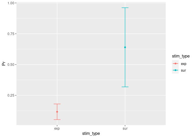
In the next step you can use this very easily generated information in order to plot the mean and according CI of the two stimulus groups:
# install.packages("ggplot2")
library(ggplot2) # Load the package.

# For plotting I use here 'ggplot2'. Look at the next section (Data visualisation magic)for further information.
ggplot(Easyinfo, aes(x=stim_type, y=Pr, colour=stim_type)) + # Here you specify the data frame you want to refer to and what should be on the x and y axes...
    geom_errorbar(aes(ymin=Pr-ci, ymax=Pr+ci), width=.1) + # Add here the CI.
    geom_line() + # This specifies that we want a simple line.
    geom_point() # But with a dot for the mean please...
## `geom_line()`: Each group consists of only one observation.
## ℹ Do you need to adjust the group aesthetic?
Another very easy way to get the same plot (but with less info and way uglier):
# install.packages("gplots")
library(gplots)
plotmeans(Pr ~ stim_type, data = example5)
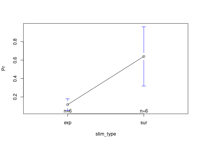
# But this is really only for the lazy ppl - stick with the 1st version if possible.
Within-subjects Design
One way to construct CIs in within-subjects designs was proposed by Cousineau (2005) and was advanced by Morey (2005). His approach suggests to normalize the data by subtracting the participant’s mean from each observation. Then, the normalized data should be used to build confidence intervals with a similar method as for between subjects which also takes the number of observations into account.
A handy way to calculate the within-subjects CI based on Cousineau is using the function cm.ci from the package tkmisc. The only requirement here is that your data are in a wide format and contain only the values of the two conditions. In this example we can use the data frame example5_wide:
# install.packages("remotes")
# remotes::install_github("TKoscik/tk.r.misc")
library(tkmisc)

CI_within = example5_wide
CI_within = CI_within[,-1] # Remove the participant column so that only the columns with the values remain in the data frame.

CI_within = as.data.frame(cm.ci(CI_within, conf.level = 0.95, difference = TRUE)) # Apply the function and put the results in a data frame.
CI_within = tibble::rownames_to_column(CI_within, "stim_type") # Change "column 0" (contains the row names and is not really a column) to a real column. We need that later for the visualisation.
CI_within$Pr = Easyinfo$Pr # Add the mean values. Also needed for the visuals.
CI_within
##   stim_type       lower     upper        Pr
## 1       exp -0.04206084 0.2753942 0.1166667
## 2       sur  0.48127250 0.7987275 0.6400000
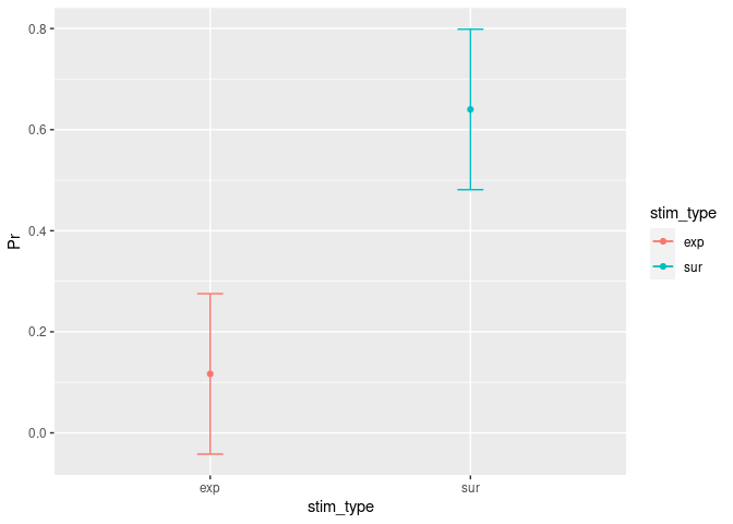
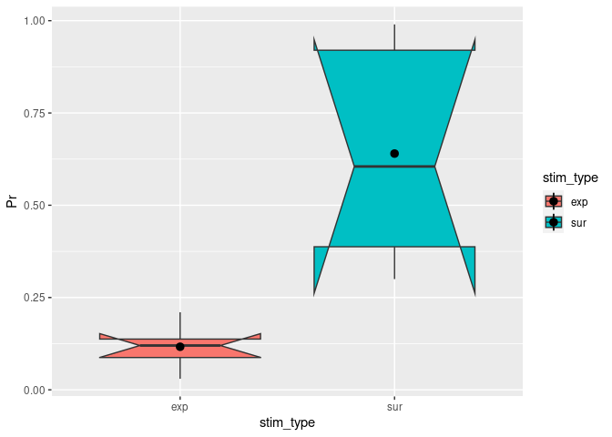
Of course we want to visually inspect these new CIs:
ggplot(CI_within, aes(x=stim_type, y=Pr, colour=stim_type)) +
  geom_errorbar(aes(ymin=lower, ymax=upper), width=.1) + # Add here the CI.
  geom_line() + # This specifies that we want a simple line.
  geom_point() # But with a dot for the mean please...
## `geom_line()`: Each group consists of only one observation.
## ℹ Do you need to adjust the group aesthetic?
Data visualisation magic
For plotting I recommend the package ggplot2 which has many helpful functions for data visualization and it also gives you the freedom to individualize the plots and to change the parameters the way you want.
Boxplots
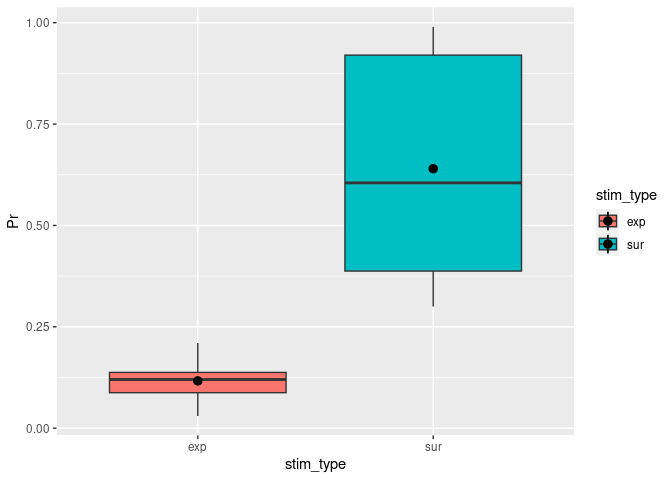
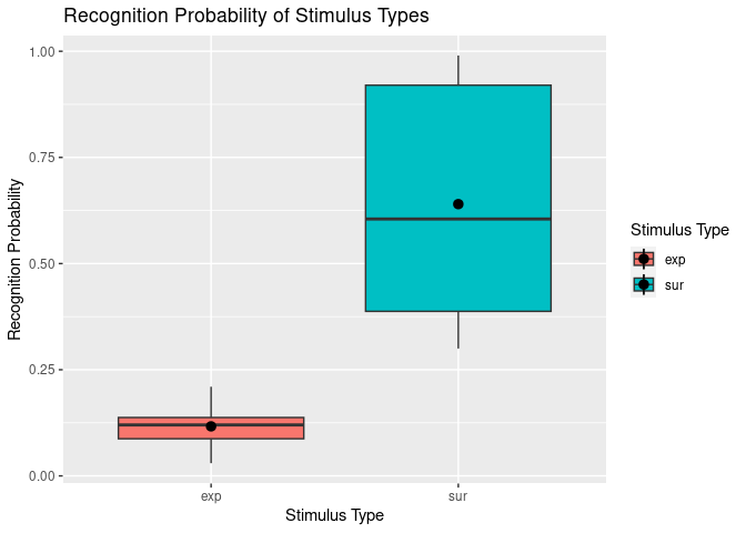
Other than the plot before, a boxplot will show you by default the median as well as the first and third quartiles (the 25th and 75th percentiles).
ggplot(example5, aes(stim_type, Pr, fill=stim_type)) + # `fill=` assignes different colors to the boxplots based on the condition.
  geom_boxplot() + # The actual function for a boxplot.
  stat_summary(fun = "mean") # It might be helpful to add the mean here as a dot.
## Warning: Removed 2 rows containing missing values (`geom_segment()`).
You can change notch to TRUE. This will give you roughly a 95% CI around the median. This is usually used to compare groups and if the boxes do not overlap you can assume that there is a difference between the two medians.
ggplot(example5, aes(stim_type, Pr, fill=stim_type)) + # `fill=` assigns different colors to the boxplots based on the condition.
  geom_boxplot(notch = TRUE) + # The actual function for a boxplot.
  stat_summary(fun = "mean") # It might be helpful to add the mean here as a dot.
## Notch went outside hinges
## ℹ Do you want `notch = FALSE`?
## Notch went outside hinges
## ℹ Do you want `notch = FALSE`?
## Warning: Removed 2 rows containing missing values (`geom_segment()`).
Adding titles and labels
Awesome – we’ve now got a plot clearly comparing the recognition probability (Pr) of our two different stimulus types. Now that we have that, we might also want to change the axis labels and legend titles to something prettier and more descriptive than the original variable names. We might also want to add a title.
One way of achieving this is by using ggplot’s labs() function. We can simply “add” this to our existing plotting code. For example:
ggplot(example5, aes(stim_type, Pr, fill=stim_type)) +
  geom_boxplot() +
  stat_summary(fun = "mean") +
  labs(title = "Recognition Probability of Stimulus Types", # This bit adds the titles.
       fill = "Stimulus Type",
       x = "Stimulus Type",
       y = "Recognition Probability"
  )
## Warning: Removed 2 rows containing missing values (`geom_segment()`).
However, you will notice that this is not completely satisfactory for our x-axis and legend, since the variable stim_type that is involved here has the discrete levels “exp” and “sur” that also need to be renamed.
This brings us to a second method of adding labels and titles which allows more fine-tuning. Here, we use scale_x_discrete() and scale_fill_discrete() to customise our x-axis and “fill” (i.e., colour fill legend) respectively.
ggplot(example5, aes(stim_type, Pr, fill=stim_type)) +
  geom_boxplot() +
  stat_summary(fun = "mean") +
  labs(title = "Recognition Probability of Stimulus Types",
       y = "Recognition Probability") + # Keep labs() function for main title and y axis since they work fine.
  scale_x_discrete(
    "Stimulus Type", # x axis title
    labels = c("exp" = "Expected", "sur" = "Surprising") # Change tick mark labels, using syntax OLD NAME = NEW NAME. Note that order specified here does not change order of display.
  ) +
  scale_fill_discrete(
   "Stimulus Type", # legend title
   labels = c("exp" = "Expected", "sur" = "Surprising")  # Change legend labels, using syntax OLD NAME = NEW NAME.
  )
## Warning: Removed 2 rows containing missing values (`geom_segment()`).
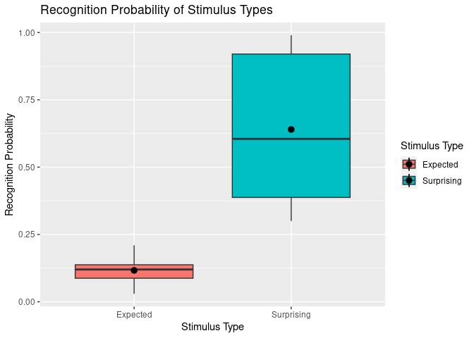
Now we have plots that make reasonable sense for any reader from a quick glance, hurrah!
Of course, there are many, many other ways to customise your data visualisation to your heart’s content – including changing background colours, text size and positions of axis labels and titles, and using a colourblind-friendly colour scheme. Some of these things can be very handy, for example, to produce APA-formatted figures suitable for inclusion in theses and papers.
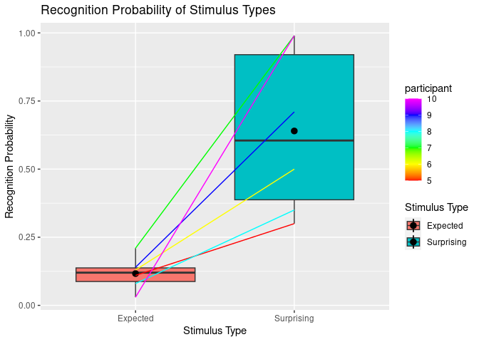
Spaghetti plots
Sometimes we want to visualise longitudinal data or we want to show which datapoints in two different conditions belong to the same participant. Therefore, we just add the geom_line() extension to what we already have created.
BUT keep in mind that too many lines (>6) can be confusing. In that case you might consider to create separate plots.
ggplot(example5, aes(stim_type, Pr, fill=stim_type)) +
  geom_boxplot() +
  stat_summary(fun = "mean") +
  labs(title = "Recognition Probability of Stimulus Types",
       y = "Recognition Probability") + # Keep labs() function for main title and y axis since they work fine.
  scale_x_discrete(
    "Stimulus Type", # x axis title
    labels = c("exp" = "Expected", "sur" = "Surprising") # Change tick mark labels, using syntax OLD NAME = NEW NAME. Note that order specified here does not change order of display.
  ) +
  scale_fill_discrete(
   "Stimulus Type", # legend title
   labels = c("exp" = "Expected", "sur" = "Surprising")  # Change legend labels, using syntax OLD NAME = NEW NAME.
  ) +
  geom_line(aes(group=participant, color=participant)) + # This is the relvant part for the spaghettis.
  scale_colour_gradientn(colours=rainbow(6)) # You can specify the color palette you want to use for the lines.
## Warning: Removed 2 rows containing missing values (`geom_segment()`).
Fancy Barplots
Barplots are convenient if you have for example a categorical variable and another one that represents the amount/number of something. Let’s assume we have 12 participants and we want to visualise how many of them chose an “Otter” as their favourite animal:
example6 = setNames(data.frame(matrix(ncol = 2, nrow = 12))
                    , c("participant", "animal"))
example6$participant = (1:12)
example6$animal = c("Otter",
                 "Lama",
                 "Otter",
                 "Otter",
                 "Lama",
                 "Lama",
                 "Otter",
                 "Bumblebee",
                 "Duck",
                 "Otter",
                 "Otter",
                 "Duck")
example6
##    participant    animal
## 1            1     Otter
## 2            2      Lama
## 3            3     Otter
## 4            4     Otter
## 5            5      Lama
## 6            6      Lama
## 7            7     Otter
## 8            8 Bumblebee
## 9            9      Duck
## 10          10     Otter
## 11          11     Otter
## 12          12      Duck
ggplot(example6, aes(animal, fill=animal)) +
  geom_bar() + # This gives you the barplot.
  labs(title = "Favourite Animal Rating",
       y = "Number") +
  scale_x_discrete(
    "Animal") +
  scale_fill_discrete(
   "Animal")
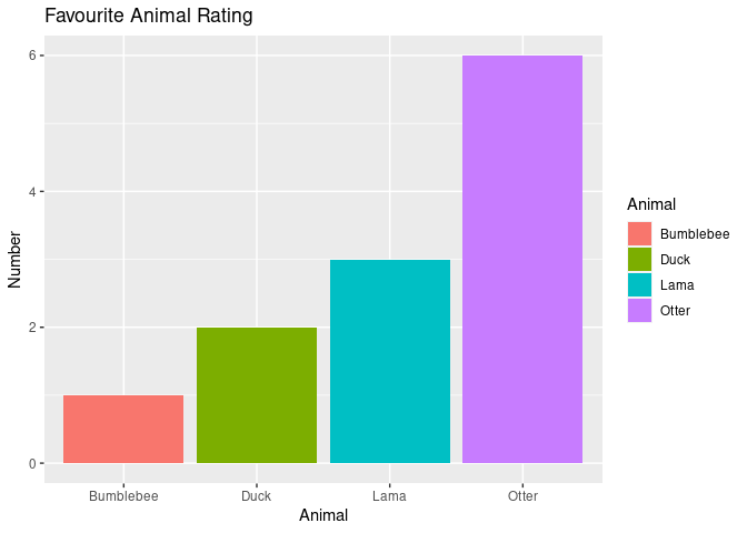
Nice!! – naturally, the Otter is clearly the most favourite animal!
Visualizing correlations with scatter plots
To demonstrate how we can visualize correlation, let us consider a second continuous variable – reaction time (rt) – in addition to our existing continuous variable Pr.
example7 <- example5
example7$rt <- c(1303,
                900,
                1193,
                1000,
                1090,
                690,
                1393,
                1121,
                970,
                988,
                1440,
                793)
example7
##    participant stim_type   Pr   rt
## 1            5       exp 0.11 1303
## 2            5       sur 0.30  900
## 3            6       exp 0.13 1193
## 4            6       sur 0.50 1000
## 5            7       exp 0.21 1090
## 6            7       sur 0.99  690
## 7            8       exp 0.08 1393
## 8            8       sur 0.35 1121
## 9            9       exp 0.14  970
## 10           9       sur 0.71  988
## 11          10       exp 0.03 1440
## 12          10       sur 0.99  793
Let’s say that we are interested in assessing whether participants’ recognition probability are correlated with their reaction time. An easy way to get a glimpse of this is using a scatterplot, by using geom_point().
ggplot(example7, aes(x=Pr , y=rt)) +
  geom_point() # Makes a scatter plot using x and y variables specified in aes().
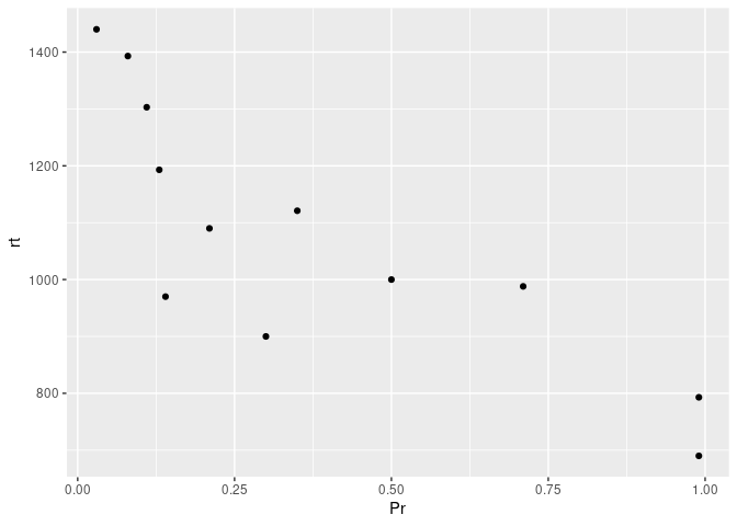
Okay, it looks like maybe something is going on here. While we could try and fit a single regression line through the above data points, it could also be more informative to see whether this relationship differs by some condition – for instance, stimulus type in our case.
ggplot(example7, aes(x=Pr, y=rt, color=stim_type, shape=stim_type)) +
  geom_point() +
  geom_smooth(method=lm, aes(fill=stim_type))
## `geom_smooth()` using formula = 'y ~ x'
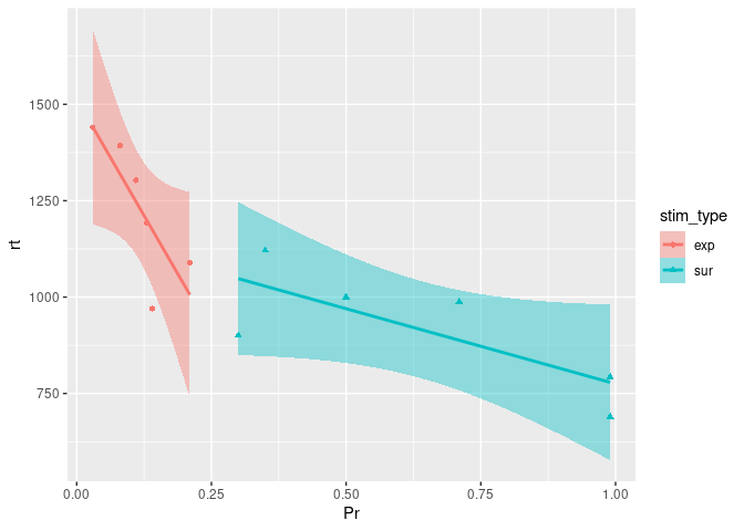
As we can see here, this visualization is quite informative, reflecting that the correlation between recognition probability and reaction time is of the same direction between the two stimulus types, and also echoing the previous boxplots that revealed recognition probability to be higher for expected stimuli than for surprising stimuli.
Here, taking a closer look at the relationship between our two continuous variables assessed, revealed that they were of a similar nature between the levels of our condition (stimulus type). That is, for both stimulus conditions, Pr and rt were negatively correlated, as was congruent with the overall relationship suggested by our first scatterplot.
In less straightforward cases, simply assessing relationships between two variables without considering subgroups, as we’d done in the first scatterplot, can be misleading (See Simpson’s Paradox). Such scenarios highlight why it can be useful – and important – to break down your visualisation by subgroups through harnessing the power of R!
V. Inferential analysis
Before starting data analysis, it is very important to check if statistical assumptions are met. Yes, okay… but why? the answer is that the so called “parametric tests” (e.g., ANOVA, t-test, regression, etc.) require that data are within certain “parameters” in order for the analyses to be accurate. The most important assumptions are:
- Normality: data should be normally distributed.
- Homogeneity of variance: variance on each group tested should be more or less equal.
Before starting, let’s create some fake data. Let’s assume that we have reasons to believe that participants remember better images of warm food rather that images of cold food. We might want to show them images of cold and warm food (within-participants variable). In addition, we want to know whether this effect changes depending on whether a participant has already eaten or not. Therefore, we assign participants to two groups: hungry and not-hungry. Finally, we test them through a recognition test. Let’s simulate!
(!! Nerd Alert!! The following procedure shows how to simulate and thus can be skipped… unless you are very interested in it)
# Set seed.
set.seed(234634)
# First, simulate recognition for hungry: the first 30 are for cold, the other 30 for warm food.
recog_perf_H<-c(rnorm(30, mean=0.60, sd=0.13), rnorm(30, mean=0.75, sd=0.12))
# Now for not hungry.
recog_perf_nH<-c(rnorm(30, mean=0.50, sd=0.14), rnorm(30, mean=0.60, sd=0.15))
# Merge both.
recog_perf<-c(recog_perf_H, recog_perf_nH)
# Create condition variable.
condition<-rep(c("cold", "warm"), each=30, times=2)
# Participant variable.
participant<-c(rep(c(1:30), times=2), rep(31:60, times=2))
group<-rep(c("hungry", "not hungry"), each=60)

# Bind it.
data_food<-data.frame(participant, condition, recog_perf, group)

# Create also a continuous variable indicating participants' working memory performance ("wm").
# We are assuming that it is correlated to the recognition performance.
wm<-vector()
for (n in 1:length(unique(participant))){
wm[n]<-mean(data_food$recog_perf[data_food$participant==data_food$participant[n]])+rnorm(1,mean=0.10, sd=0.02)
}
# Order according to participants.
data_food<-data_food[order(data_food$participant),]
# Attach the wm variable.
data_food$wm<-rep(wm, each=2)
# Check the structure of the data.
str(data_food)
## 'data.frame':	120 obs. of  5 variables:
##  $ participant: int  1 1 2 2 3 3 4 4 5 5 ...
##  $ condition  : chr  "cold" "warm" "cold" "warm" ...
##  $ recog_perf : num  0.37 0.68 0.678 0.762 0.607 ...
##  $ group      : chr  "hungry" "hungry" "hungry" "hungry" ...
##  $ wm         : num  0.663 0.663 0.826 0.826 0.8 ...
# Check the format of the data:
head(data_food)
##    participant condition recog_perf  group        wm
## 1            1      cold  0.3701675 hungry 0.6630468
## 31           1      warm  0.6795923 hungry 0.6630468
## 2            2      cold  0.6779541 hungry 0.8260525
## 32           2      warm  0.7617480 hungry 0.8260525
## 3            3      cold  0.6066051 hungry 0.8002971
## 33           3      warm  0.8200754 hungry 0.8002971
# Let us look at the data:
data_food
##     participant condition recog_perf      group        wm
## 1             1      cold  0.3701675     hungry 0.6630468
## 31            1      warm  0.6795923     hungry 0.6630468
## 2             2      cold  0.6779541     hungry 0.8260525
## 32            2      warm  0.7617480     hungry 0.8260525
## 3             3      cold  0.6066051     hungry 0.8002971
## 33            3      warm  0.8200754     hungry 0.8002971
## 4             4      cold  0.4540464     hungry 0.6848700
## 34            4      warm  0.7102183     hungry 0.6848700
## 5             5      cold  0.4525917     hungry 0.6968984
## 35            5      warm  0.8072747     hungry 0.6968984
## 6             6      cold  0.7107697     hungry 0.7940126
## 36            6      warm  0.7325580     hungry 0.7940126
## 7             7      cold  0.4231543     hungry 0.6735239
## 37            7      warm  0.6741001     hungry 0.6735239
## 8             8      cold  0.7332302     hungry 0.7996366
## 38            8      warm  0.6361844     hungry 0.7996366
## 9             9      cold  0.6589959     hungry 0.8699979
## 39            9      warm  0.8425297     hungry 0.8699979
## 10           10      cold  0.8118603     hungry 0.7950518
## 40           10      warm  0.6340307     hungry 0.7950518
## 11           11      cold  0.7166698     hungry 0.7328982
## 41           11      warm  0.5267856     hungry 0.7328982
## 12           12      cold  0.6445626     hungry 0.7683372
## 42           12      warm  0.8025181     hungry 0.7683372
## 13           13      cold  0.5603714     hungry 0.8093576
## 43           13      warm  0.8372279     hungry 0.8093576
## 14           14      cold  0.6862972     hungry 0.8875440
## 44           14      warm  0.8588887     hungry 0.8875440
## 15           15      cold  0.6597363     hungry 0.7976466
## 45           15      warm  0.7621104     hungry 0.7976466
## 16           16      cold  0.6221724     hungry 0.7595080
## 46           16      warm  0.7029713     hungry 0.7595080
## 17           17      cold  0.6986523     hungry 0.8463840
## 47           17      warm  0.8556005     hungry 0.8463840
## 18           18      cold  0.6977015     hungry 0.8425226
## 48           18      warm  0.7773590     hungry 0.8425226
## 19           19      cold  0.5303337     hungry 0.7593470
## 49           19      warm  0.7456964     hungry 0.7593470
## 20           20      cold  0.5676298     hungry 0.6920881
## 50           20      warm  0.6067139     hungry 0.6920881
## 21           21      cold  0.3938138     hungry 0.6457582
## 51           21      warm  0.7079651     hungry 0.6457582
## 22           22      cold  0.5149368     hungry 0.7221189
## 52           22      warm  0.7385895     hungry 0.7221189
## 23           23      cold  0.4986928     hungry 0.7771958
## 53           23      warm  0.8619420     hungry 0.7771958
## 24           24      cold  0.4393526     hungry 0.6174584
## 54           24      warm  0.6565674     hungry 0.6174584
## 25           25      cold  0.5152447     hungry 0.6819865
## 55           25      warm  0.6365579     hungry 0.6819865
## 26           26      cold  0.5479081     hungry 0.7322531
## 56           26      warm  0.7232609     hungry 0.7322531
## 27           27      cold  0.7701120     hungry 0.8523281
## 57           27      warm  0.7327927     hungry 0.8523281
## 28           28      cold  0.7432171     hungry 0.9978315
## 58           28      warm  1.1242861     hungry 0.9978315
## 29           29      cold  0.7103051     hungry 0.8587518
## 59           29      warm  0.8088224     hungry 0.8587518
## 30           30      cold  0.3984270     hungry 0.7537614
## 60           30      warm  0.8910267     hungry 0.7537614
## 61           31      cold  0.6626482 not hungry 0.6299393
## 91           31      warm  0.5045346 not hungry 0.6299393
## 62           32      cold  0.5145876 not hungry 0.8531309
## 92           32      warm  0.5663960 not hungry 0.8531309
## 63           33      cold  0.5636475 not hungry 0.7841366
## 93           33      warm  0.8119157 not hungry 0.7841366
## 64           34      cold  0.5536680 not hungry 0.7192232
## 94           34      warm  0.7631179 not hungry 0.7192232
## 65           35      cold  0.7037965 not hungry 0.7208457
## 95           35      warm  0.3003196 not hungry 0.7208457
## 66           36      cold  0.5497271 not hungry 0.8038275
## 96           36      warm  0.6614769 not hungry 0.8038275
## 67           37      cold  0.5584065 not hungry 0.6287822
## 97           37      warm  0.9098799 not hungry 0.6287822
## 68           38      cold  0.6208255 not hungry 0.7695700
## 98           38      warm  0.7296477 not hungry 0.7695700
## 69           39      cold  0.6492774 not hungry 0.8753173
## 99           39      warm  0.8810639 not hungry 0.8753173
## 70           40      cold  0.5344712 not hungry 0.8335446
## 100          40      warm  0.9798494 not hungry 0.8335446
## 71           41      cold  0.3442439 not hungry 0.6993906
## 101          41      warm  0.6715204 not hungry 0.6993906
## 72           42      cold  0.4173514 not hungry 0.8510779
## 102          42      warm  0.4766666 not hungry 0.8510779
## 73           43      cold  0.4100487 not hungry 0.8055182
## 103          43      warm  0.6404090 not hungry 0.8055182
## 74           44      cold  0.4352504 not hungry 0.8917084
## 104          44      warm  0.4127080 not hungry 0.8917084
## 75           45      cold  0.6712228 not hungry 0.8168989
## 105          45      warm  0.3582321 not hungry 0.8168989
## 76           46      cold  0.3718020 not hungry 0.7671125
## 106          46      warm  0.6575176 not hungry 0.7671125
## 77           47      cold  0.6736324 not hungry 0.8866329
## 107          47      warm  0.6816603 not hungry 0.8866329
## 78           48      cold  0.5611509 not hungry 0.8291472
## 108          48      warm  0.6815224 not hungry 0.8291472
## 79           49      cold  0.4464589 not hungry 0.7247024
## 109          49      warm  0.6740202 not hungry 0.7247024
## 80           50      cold  0.4074223 not hungry 0.6494969
## 110          50      warm  0.7224195 not hungry 0.6494969
## 81           51      cold  0.5268512 not hungry 0.6877570
## 111          51      warm  0.5976927 not hungry 0.6877570
## 82           52      cold  0.5200971 not hungry 0.7275831
## 112          52      warm  0.6708792 not hungry 0.7275831
## 83           53      cold  0.6188257 not hungry 0.7826997
## 113          53      warm  0.6442603 not hungry 0.7826997
## 84           54      cold  0.4021081 not hungry 0.6371289
## 114          54      warm  0.9137242 not hungry 0.6371289
## 85           55      cold  0.4197974 not hungry 0.6798813
## 115          55      warm  0.5369418 not hungry 0.6798813
## 86           56      cold  0.3186018 not hungry 0.7523661
## 116          56      warm  0.7326065 not hungry 0.7523661
## 87           57      cold  0.6844472 not hungry 0.8608357
## 117          57      warm  0.3245837 not hungry 0.8608357
## 88           58      cold  0.6229062 not hungry 1.0451762
## 118          58      warm  0.2748781 not hungry 1.0451762
## 89           59      cold  0.3170245 not hungry 0.8247061
## 119          59      warm  0.7550980 not hungry 0.8247061
## 90           60      cold  0.5508814 not hungry 0.7728054
## 120          60      warm  0.5951913 not hungry 0.7728054
The data are organized into a “long format”, in which every row represents on condition of the variable repeated within participant. As the only repeated variable (“condition”) has only two levels, we have two rows for each participant.
Normality assumption
# Check the distribution of the response variable, performance (DV).
library(ggplot2)
ggplot(data_food, aes(recog_perf)) +
  geom_histogram(aes(y=..density..), colour="black", fill="white") +
  geom_density()+
  facet_grid(condition~group)
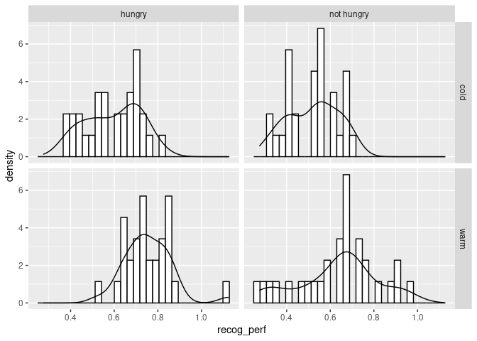
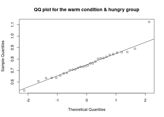
The distribution looks roughly normal. We could use a QQ plot.
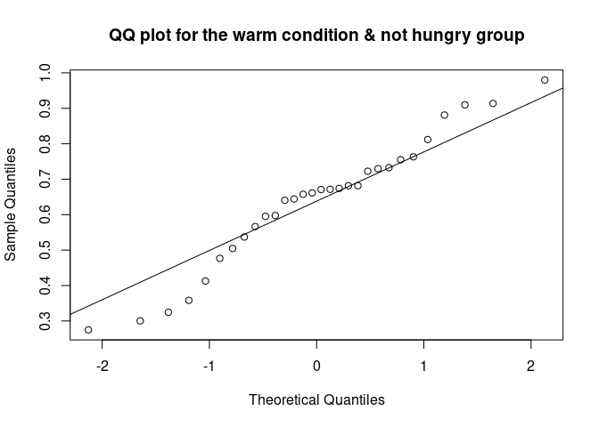
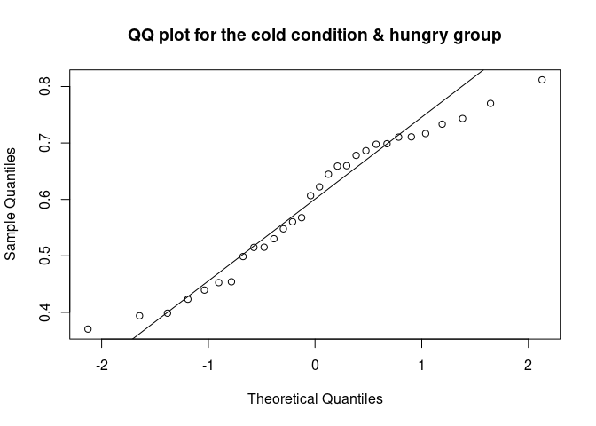
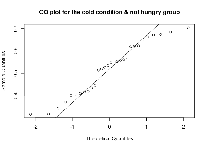
The QQ plot (quantile-quantile plot) shows the correlation between the observed data and the expected values, namely the values if data were normally distributed. If observed data are normally distributed, the QQ plot looks as a straight diagonal line. Deviations from the diagonal shows deviation from normality.
qqnorm(data_food$recog_perf[data_food$condition=="warm" & data_food$group=="hungry"], main = "QQ plot for the warm condition & hungry group")
qqline(data_food$recog_perf[data_food$condition=="warm" & data_food$group=="hungry"])
qqnorm(data_food$recog_perf[data_food$condition=="warm" & data_food$group=="not hungry"], main = "QQ plot for the warm condition & not hungry group")
qqline(data_food$recog_perf[data_food$condition=="warm" & data_food$group=="not hungry"])
qqnorm(data_food$recog_perf[data_food$condition=="cold" & data_food$group=="hungry"], main = "QQ plot for the cold condition & hungry group")
qqline(data_food$recog_perf[data_food$condition=="cold" & data_food$group=="hungry"])
qqnorm(data_food$recog_perf[data_food$condition=="cold" & data_food$group=="not hungry"], main = "QQ plot for the cold condition & not hungry group")
qqline(data_food$recog_perf[data_food$condition=="cold" & data_food$group=="not hungry"])
In order to test whether the distribution deviates from a normal distribution, we can use the Shapiro-Wilk test.
This test compares the observed vales are significantly different from normally distributed values. If the test is non-significant (p > .05), the distribution of data is not different from a normal distribution.
shapiro.test(data_food$recog_perf[data_food$condition=="warm" & data_food$group=="hungry"])
##
## 	Shapiro-Wilk normality test
##
## data:  data_food$recog_perf[data_food$condition == "warm" & data_food$group == "hungry"]
## W = 0.93816, p-value = 0.08114
shapiro.test(data_food$recog_perf[data_food$condition=="cold" & data_food$group=="hungry"])
##
## 	Shapiro-Wilk normality test
##
## data:  data_food$recog_perf[data_food$condition == "cold" & data_food$group == "hungry"]
## W = 0.94964, p-value = 0.1653
shapiro.test(data_food$recog_perf[data_food$condition=="warm" & data_food$group=="not hungry"])
##
## 	Shapiro-Wilk normality test
##
## data:  data_food$recog_perf[data_food$condition == "warm" & data_food$group == "not hungry"]
## W = 0.96162, p-value = 0.3405
shapiro.test(data_food$recog_perf[data_food$condition=="cold" & data_food$group=="not hungry"])
##
## 	Shapiro-Wilk normality test
##
## data:  data_food$recog_perf[data_food$condition == "cold" & data_food$group == "not hungry"]
## W = 0.94587, p-value = 0.131
As we can see, the four tests indicate that data does not deviate from normality. In case data are not normally distributed, we can use a transformation (square, log, inverse transformation), use a non- parametric test (e.g., Spearman correlation, Mann-Whitney for comparing two means, Kruskal-Wallis for comparing multiple means), or we can use a different distribution (binomial, multinomial, etc.).
Homogeneity of variance assumption
In addition to being normally distributed, parametric tests require that the variances of different levels of one variable should be more or less equal. In other words, the variances should be “homogeneous”.
In order to check for homogeneity fo variance, we can use the Levene test.
library(car)
# We can check first if the variance differ across food condition.
leveneTest(data_food$recog_perf, data_food$condition)
## Levene's Test for Homogeneity of Variance (center = median)
##        Df F value Pr(>F)
## group   1  0.5047 0.4788
##       118
# Then across hunger group.
leveneTest(data_food$recog_perf, data_food$group)
## Levene's Test for Homogeneity of Variance (center = median)
##        Df F value Pr(>F)
## group   1  1.4927 0.2242
##       118
The variance seems to be homogeneous across condition and group. Similar to the Levene test, we are testing the null hypothesis, that the variances are homogenous, which is the case if our test is non-significant (p>.05). Let’s run our parametric tests!
Correlation
We can start our analysis by checking whether participants’ working memory correlates with recognition performance. For a more detailed tutorial on correlation, check out pandaR.
In order to do this, we need to work on a “wide-dataset”, where every row represents a participant. We can use the reshape() function from the reshape2 package.
library(reshape2)
##
## Attaching package: 'reshape2'
## The following object is masked from 'package:tidyr':
##
##     smiths
# Create a wide dataset by aggregating performance on the participant level.
# In order to do that, we can use the reshape function.
# We need to specify the grouping variables ("idvar"), i.e. the variables that vary between participants. Those are participants' id, group, and wm. The condition that varies within participant ("timevar") is "condition".
data_food_wide<-reshape(data_food, idvar = c("participant", "group", "wm"), timevar = "condition", direction = "wide")

# Let's have a look at this dataset.
head(data_food_wide)
##   participant  group        wm recog_perf.cold recog_perf.warm
## 1           1 hungry 0.6630468       0.3701675       0.6795923
## 2           2 hungry 0.8260525       0.6779541       0.7617480
## 3           3 hungry 0.8002971       0.6066051       0.8200754
## 4           4 hungry 0.6848700       0.4540464       0.7102183
## 5           5 hungry 0.6968984       0.4525917       0.8072747
## 6           6 hungry 0.7940126       0.7107697       0.7325580
# As you can see, we have two columns indicating "recog_perf.warm" for warm condition, and "recog_perf.cold" for cold condition.

# We want to aggregate it by averaging within participant, to have one variable indicating the recognition performance at the participant level.
# We can use the useful "rowMeans" function.
data_food_wide$recog_perf_avg<-rowMeans(data_food_wide[c("recog_perf.warm", "recog_perf.cold")])

# Check if wm is normally distributed.
shapiro.test(data_food_wide$wm)
##
## 	Shapiro-Wilk normality test
##
## data:  data_food_wide$wm
## W = 0.96993, p-value = 0.1447
# Do the same for the aggregated recognition performance.
shapiro.test(data_food_wide$recog_perf_avg)
##
## 	Shapiro-Wilk normality test
##
## data:  data_food_wide$recog_perf_avg
## W = 0.97621, p-value = 0.2898
# They are both normally distributed. Let's do the correlation.
cor.test(data_food_wide$recog_perf_avg, data_food_wide$wm)
##
## 	Pearson's product-moment correlation
##
## data:  data_food_wide$recog_perf_avg and data_food_wide$wm
## t = 2.2897, df = 58, p-value = 0.02569
## alternative hypothesis: true correlation is not equal to 0
## 95 percent confidence interval:
##  0.03667974 0.50493156
## sample estimates:
##       cor
## 0.2879228
There is a significant correlation between participants’ working memory and their recognition performance: Person’s r = 0.29, p < .026.
Regression
With regression we also explore relationships between variables. Unlike correlation, regression assumes that there are a response variable (or dependent variable, or outcome) and one or several predictors (or independent variables). It also allows to make prediction, thanks to the coefficients that it returns.
A more detailed tutorial on regression analysis can also be found on pandaR, where there’s a special tutorial on it.
Let’s consider our working memory - recognition relationship as a regression.
# R uses the "lm" (Linear Model) function to compute regression.
regres<-lm(recog_perf_avg~wm, data=data_food_wide)
# On the left side of the "~" there is the dependent variable, on the right the predictor(s).
# Let's have a look at the output.
summary(regres)
##
## Call:
## lm(formula = recog_perf_avg ~ wm, data = data_food_wide)
##
## Residuals:
##      Min       1Q   Median       3Q      Max
## -0.26837 -0.05103  0.01087  0.07627  0.23227
##
## Coefficients:
##             Estimate Std. Error t value Pr(>|t|)
## (Intercept)   0.3690     0.1134   3.254   0.0019 **
## wm            0.3332     0.1455   2.290   0.0257 *
## ---
## Signif. codes:  0 '***' 0.001 '**' 0.01 '*' 0.05 '.' 0.1 ' ' 1
##
## Residual standard error: 0.09802 on 58 degrees of freedom
## Multiple R-squared:  0.0829,	Adjusted R-squared:  0.06709
## F-statistic: 5.243 on 1 and 58 DF,  p-value: 0.02569
The intercept is not informative in this case: it just tells us that when wm is 0, recognition performance is 0.369, and that this value is significantly different from 0. The estimate for “wm” tells us that after one unit change in our predictor (working memory), the response (recognition memory in %) increases by 0.33. This effect is significant.
t-test
We use t-tests to compare differences between two groups or conditions. In our food_data we have two groups and two conditions: the hungry - not hungry groups vary between participants, while the warm - cold conditions vary within-participants. Let’s test if they differ! We can start from the between-participants variable.
t.test(recog_perf_avg~group, data = data_food_wide)
##
## 	Welch Two Sample t-test
##
## data:  recog_perf_avg by group
## t = 4.0861, df = 57.953, p-value = 0.0001366
## alternative hypothesis: true difference in means between group hungry and group not hungry is not equal to 0
## 95 percent confidence interval:
##  0.04854198 0.14177779
## sample estimates:
##     mean in group hungry mean in group not hungry
##                0.6745251                0.5793652
There is a significant difference between the groups, so that the hungry group better recognized the images.
The t-test, like the ANOVA, can be considered as a special case of regression, in which the predictor (IV) is categorical.
R automatically dummy-codes the two group as “0” and “1” and returns the difference between the two.
Therefore, we could run a t-test by using the lm() function as we have already done for regression
t_test_as_reg<-lm(recog_perf_avg~group, data = data_food_wide)

summary(t_test_as_reg)
##
## Call:
## lm(formula = recog_perf_avg ~ group, data = data_food_wide)
##
## Residuals:
##       Min        1Q    Median        3Q       Max
## -0.155386 -0.064655 -0.009141  0.054885  0.259226
##
## Coefficients:
##                 Estimate Std. Error t value Pr(>|t|)
## (Intercept)      0.67453    0.01647  40.961  < 2e-16 ***
## groupnot hungry -0.09516    0.02329  -4.086 0.000136 ***
## ---
## Signif. codes:  0 '***' 0.001 '**' 0.01 '*' 0.05 '.' 0.1 ' ' 1
##
## Residual standard error: 0.0902 on 58 degrees of freedom
## Multiple R-squared:  0.2235,	Adjusted R-squared:  0.2101
## F-statistic:  16.7 on 1 and 58 DF,  p-value: 0.0001365
# The t-value and p-value are the same as the t-test that we did before.
The only difference with the test that we ran before is that the sign of the t-value in the lm was negative. This occurs because the values that are shown refer to the difference between the “not hungry” condition and the “hungry” condition, the latter being the reference level (R automatically assigns reference level according to alphabetical order).
Now we can compare the within-participants variable: condition (warm vs. cold) In this case we have to use a paired sample t-test. We can use the t-test function and specify that the data are paired.
# Subset the variable to extract the data.
t.test(data_food_wide$recog_perf.warm, data_food_wide$recog_perf.cold, paired = TRUE)
##
## 	Paired t-test
##
## data:  data_food_wide$recog_perf.warm and data_food_wide$recog_perf.cold
## t = 5.2523, df = 59, p-value = 2.159e-06
## alternative hypothesis: true mean difference is not equal to 0
## 95 percent confidence interval:
##  0.08604487 0.19195630
## sample estimates:
## mean difference
##       0.1390006
# This t-test is considering that each case is "paired" with the other, meaning that it is coming from the same participant.

# In order to understand the direction of the difference, let's get the means of the two conditions.
by(data_food$recog_perf, data_food$condition, FUN = mean)
## data_food$condition: cold
## [1] 0.5574449
## ------------------------------------------------------------------------
## data_food$condition: warm
## [1] 0.6964455
Warm food is remembered better than cold food. We could also consider the paired-sample t-test as a regression, but in this case would be a bit more difficult. In fact, in this case we have to take into account the dependency in the data, and this is usually done by adding random effects to the normal regression. But we can look into it later on.
One-way ANOVA
Now that we know how to compare two means, we can consider cases in which we have more than two. This is usually done with an ANOVA. To find out more about ANOVAs and contrasts, have a look at the pandaR tutorial!
(!! Nerd Alert !!) We need to create a third group in our data. The following section is not important and can be skipped, unless you are really interested.
# We can create a third group of "super hungry" people that are just starving.
recog_perf_sH<-c(rnorm(30, mean=0.40, sd=0.13), rnorm(30, mean=0.50, sd=0.12))

# Create condition variable.
condition<-rep(c("cold", "warm"), each=30)
# Participant variable.
participant<-rep((61:90), times=2)
# Group variable.
group<-rep("super hungry", times=30)

# Bind it.
data_food_sH<-data.frame(participant, condition, "recog_perf" = recog_perf_sH, group)

# Working memory.
wm<-vector()
for (n in 1:length(unique(participant))){
  wm[n]<-mean(data_food_sH$recog_perf[data_food_sH$participant==data_food_sH$participant[n]])+rnorm(1,mean=0.10, sd=0.02)
}

# Order according to participants.
data_food_sH<-data_food_sH[order(data_food_sH$participant),]
# Attach the wm variable.
data_food_sH$wm<-rep(wm, each=2)

# Attach to the previous dataframe.
data_food<-rbind(data_food, data_food_sH)
head(data_food)
##    participant condition recog_perf  group        wm
## 1            1      cold  0.3701675 hungry 0.6630468
## 31           1      warm  0.6795923 hungry 0.6630468
## 2            2      cold  0.6779541 hungry 0.8260525
## 32           2      warm  0.7617480 hungry 0.8260525
## 3            3      cold  0.6066051 hungry 0.8002971
## 33           3      warm  0.8200754 hungry 0.8002971
# Re-create the dataframe in wide format.
data_food_wide<-reshape(data_food, idvar = c("participant", "group", "wm"), timevar = "condition", direction = "wide")

data_food_wide$recog_perf_avg<-rowMeans(data_food_wide[c("recog_perf.warm", "recog_perf.cold")])
head(data_food_wide)
##   participant  group        wm recog_perf.cold recog_perf.warm recog_perf_avg
## 1           1 hungry 0.6630468       0.3701675       0.6795923      0.5248799
## 2           2 hungry 0.8260525       0.6779541       0.7617480      0.7198511
## 3           3 hungry 0.8002971       0.6066051       0.8200754      0.7133403
## 4           4 hungry 0.6848700       0.4540464       0.7102183      0.5821324
## 5           5 hungry 0.6968984       0.4525917       0.8072747      0.6299332
## 6           6 hungry 0.7940126       0.7107697       0.7325580      0.7216639
Okay, now let’s compare the three groups (hungry, not hungry, super hungry) in our wide format dataset (data_food_wide). We can use the aov() function. Another popular way to run ANOVAs is by using the ez() package.
# Let's run a levene test first.
leveneTest(data_food_wide$recog_perf_avg, data_food_wide$group, center = mean)
## Warning in leveneTest.default(data_food_wide$recog_perf_avg, data_food_wide$group, :
## data_food_wide$group coerced to factor.
## Levene's Test for Homogeneity of Variance (center = mean)
##       Df F value Pr(>F)
## group  2  0.0545  0.947
##       87
# Since it is non-significant, the variances of the two groups are similar.
anova_betw<-aov(recog_perf_avg~group, data=data_food_wide)

# Let's see the results.
summary(anova_betw)
##             Df Sum Sq Mean Sq F value Pr(>F)
## group        2 0.9684  0.4842   58.91 <2e-16 ***
## Residuals   87 0.7151  0.0082
## ---
## Signif. codes:  0 '***' 0.001 '**' 0.01 '*' 0.05 '.' 0.1 ' ' 1
# The "summary" function returns the "omnibus" test, testing whether the recognition performance varies as a function of the hungry group. If we want to have an idea on the differences between the different conditions, we can run the ANOVA as a regression, by using the "lm" function.
LM_betw<-lm(recog_perf_avg~group, data=data_food_wide)
summary(LM_betw)
##
## Call:
## lm(formula = recog_perf_avg ~ group, data = data_food_wide)
##
## Residuals:
##       Min        1Q    Median        3Q       Max
## -0.157293 -0.064689 -0.009141  0.054474  0.259226
##
## Coefficients:
##                   Estimate Std. Error t value Pr(>|t|)
## (Intercept)        0.67453    0.01655  40.750  < 2e-16 ***
## groupnot hungry   -0.09516    0.02341  -4.065 0.000105 ***
## groupsuper hungry -0.25162    0.02341 -10.749  < 2e-16 ***
## ---
## Signif. codes:  0 '***' 0.001 '**' 0.01 '*' 0.05 '.' 0.1 ' ' 1
##
## Residual standard error: 0.09066 on 87 degrees of freedom
## Multiple R-squared:  0.5752,	Adjusted R-squared:  0.5655
## F-statistic: 58.91 on 2 and 87 DF,  p-value: < 2.2e-16
The output of the ANOVA as regression analysis shows three coefficients. The intercept represents the mean recognition performance for the baseline condition (group “hungry”, coded as baseline because it is the first in alphabetical order). The “groupnot hungry” represents the difference between recognition performance of the group “not hungry” and recognition performance of the group “hungry” (baseline). Participants who are hungry perform a bit worse than participants that are not hungry, and the difference in performance is significant. Finally, the coefficient “groupsuper hungry” represents the difference in recognition performance between the superhungry group and the hungry group. The super hungry performed significantly worse than the hungry ones… probably at some point the hunger becomes really distracting :)
But what about the difference between the super hungry and not hungry groups? If we are interested in it, we can change the reference category.
# Let's make the "super hungry" group the reference level.
#data_food_wide$group<-relevel(data_food_wide$group, ref = "super hungry")

# Run the anova again.
LM_betw_sH<-lm(recog_perf_avg~group, data=data_food_wide)

summary(LM_betw_sH)
##
## Call:
## lm(formula = recog_perf_avg ~ group, data = data_food_wide)
##
## Residuals:
##       Min        1Q    Median        3Q       Max
## -0.157293 -0.064689 -0.009141  0.054474  0.259226
##
## Coefficients:
##                   Estimate Std. Error t value Pr(>|t|)
## (Intercept)        0.67453    0.01655  40.750  < 2e-16 ***
## groupnot hungry   -0.09516    0.02341  -4.065 0.000105 ***
## groupsuper hungry -0.25162    0.02341 -10.749  < 2e-16 ***
## ---
## Signif. codes:  0 '***' 0.001 '**' 0.01 '*' 0.05 '.' 0.1 ' ' 1
##
## Residual standard error: 0.09066 on 87 degrees of freedom
## Multiple R-squared:  0.5752,	Adjusted R-squared:  0.5655
## F-statistic: 58.91 on 2 and 87 DF,  p-value: < 2.2e-16
The super hungry group performed worse than the not hungry group. You could also use different contrasts (repeated, helmert, etc.) or make your own contrasts. See here how.
Repeated measures ANOVA
We have seen how to run an ANOVA when our dependent variable varies between participants. But what about within-participants variables?
There is also a tutorial on pandaR on this topic, including contrasts, how convenient!
First, we need to create a third condition. Let’s imagine that we are also showing images of frozen food.
(!! Nerd Alert !!) You know what I mean.
recog_perf_H<-rnorm(30, mean=0.50, sd=0.13)
# Now for not hungry.
recog_perf_nH<-rnorm(30, mean=0.40, sd=0.14)

recog_perf_sH<-rnorm(30, mean=0.30, sd=0.13)

# Merge both.
recog_perf<-c(recog_perf_H, recog_perf_nH,recog_perf_sH)
# Create condition variable.
condition<-rep("frozen", times = 90)
# Participant variable.
participant<-1:90
group<-rep(c("hungry", "not hungry", "super hungry"), each=30)

# Bind it.
data_food_froz<-data.frame(participant, condition, recog_perf, group)

# Create working memory.
for (n in 1:length(unique(participant))){
  wm[n]<-mean(data_food_froz$recog_perf[data_food_froz$participant==data_food_froz$participant[n]])+rnorm(1,mean=0.10, sd=0.02)
}
# Order according to participants.
data_food_froz<-data_food_froz[order(data_food_froz$participant),]
# Attach the wm variable.
data_food_froz$wm<-wm

# Finally, attach the so-created data to the dataframe.
data_food<-rbind(data_food, data_food_froz)

# Order it according to participants.
data_food<-data_food[order(data_food$participant),]

# Let's have a look at the data.
head(data_food)
##     participant condition recog_perf  group        wm
## 1             1      cold  0.3701675 hungry 0.6630468
## 31            1      warm  0.6795923 hungry 0.6630468
## 123           1    frozen  0.3512959 hungry 0.4174005
## 2             2      cold  0.6779541 hungry 0.8260525
## 32            2      warm  0.7617480 hungry 0.8260525
## 212           2    frozen  0.5485068 hungry 0.6709165
You can see that we now have three different measures for each participant, corresponding to the three food conditions: cold, warm, and frozen.
Now we want to check whether the recognition performance varies as a function of these three food conditions, that are repeated withing participants. In order to do that, we can use the “ezAnova” function, from the package “ez”
library(ez)
# Convert participant variable as factor.
data_food$participant<-as.factor(data_food$participant)
anova_within<-ezANOVA(data = data_food, # Dataframe.
                 dv = .(recog_perf), # Dependent variable. This functions requires to place the name of each variable within .()
                 wid = .(participant), # Variable that identifies participants.
                 within = .(condition), # Independent variable.
                 detailed = T
                 )

# Let's call the model.
anova_within
## $ANOVA
##        Effect DFn DFd       SSn      SSd          F            p p<.05       ges
## 1 (Intercept)   1  89 68.997174 4.181903 1468.41017 4.211490e-57     * 0.9045323
## 2   condition   2 178  2.295248 3.100315   65.88912 3.835747e-22     * 0.2396508
##
## $`Mauchly's Test for Sphericity`
##      Effect         W         p p<.05
## 2 condition 0.9633512 0.1934302
##
## $`Sphericity Corrections`
##      Effect       GGe        p[GG] p[GG]<.05       HFe        p[HF] p[HF]<.05
## 2 condition 0.9646468 1.888423e-21         * 0.9856153 7.336609e-22         *
The results show that recognition performance significantly differed across conditions.
The ezAnova() function also runs a “Mauchly test for Sphericity”, and corrected results in case it turns out to be significant.
But what about contrasts?
# We could use the following syntax to run pairwise, bonferroni corrected, contrasts.
pairwise.t.test(data_food$recog_perf, data_food$condition, paired = TRUE,
p.adjust.method = "bonferroni")
##
## 	Pairwise comparisons using paired t tests
##
## data:  data_food$recog_perf and data_food$condition
##
##        cold    frozen
## frozen 2.3e-06 -
## warm   8.1e-08 < 2e-16
##
## P value adjustment method: bonferroni
What we see here is a matrix with the p-values of the contrasts. You can see that all the three pairwise contrasts are significant.
We could also consider the repeated measure ANOVA as a regression. In order to do so, we need to add some more information to the model, as we need to account for the dependency of the data within-participants and conditions. This is usually done by adding random effects to the regression model. The so-obtained model is called “Linear Mixed Model”, LMM, or multilevel regression. There are also other ways to define these kind of models, but I let you find them out! The package used to run LMM is “lme4”.
library(lme4)
library(lmerTest) # We also need this package to show the p-values.

# The function we are using is "lmer" function. It is very similar to the lm function, with the only difference that it requires specification of the random effects.
LLM_within<-lmer(recog_perf ~ condition # So far it is the same as the lm function. Now we need to add the random effects.
          + (1| participant),  # We are specifying that the data are nested within participants (random intercept of participants)
          data = data_food
          )

summary(LLM_within)
## Linear mixed model fit by REML. t-tests use Satterthwaite's method ['lmerModLmerTest']
## Formula: recog_perf ~ condition + (1 | participant)
##    Data: data_food
##
## REML criterion at convergence: -221.9
##
## Scaled residuals:
##      Min       1Q   Median       3Q      Max
## -2.51484 -0.54316  0.07976  0.60180  2.64510
##
## Random effects:
##  Groups      Name        Variance Std.Dev.
##  participant (Intercept) 0.009857 0.09928
##  Residual                0.017418 0.13198
## Number of obs: 270, groups:  participant, 90
##
## Fixed effects:
##                  Estimate Std. Error        df t value Pr(>|t|)
## (Intercept)       0.49420    0.01741 211.70141  28.389  < 2e-16 ***
## conditionfrozen  -0.09552    0.01967 178.00000  -4.855 2.62e-06 ***
## conditionwarm     0.12947    0.01967 178.00000   6.581 5.05e-10 ***
## ---
## Signif. codes:  0 '***' 0.001 '**' 0.01 '*' 0.05 '.' 0.1 ' ' 1
##
## Correlation of Fixed Effects:
##             (Intr) cndtnf
## conditnfrzn -0.565
## conditinwrm -0.565  0.500
Mixed designs (within/between factors)
We might have a design in which we are interested in the effects of variables that vary within-participants and between-participants. In this case, we should include the main effects of the variables (and their interaction) in one single model. In our example, we might be interested in the interaction between the food condition (within-participant variable) and participants’ group (between-participants condition). Does the effect of food condition (warm, cold, frozen) vary as a function of participants’ hunger?
In order to find it out, we can consider this analysis either as a mixed-model ANOVA, or as a multiple regression with random effects (Linear Mixed Model, LMM).
Let’s start with the former.
# This analysis is the same as our previous ezAnova example, with the only difference that we are adding a between-participants variable(group).
anova_mixed<-ezANOVA(data = data_food, # Dataframe.
                 dv = .(recog_perf), # Dependent variable. This functions requires to place the name of each variable within .()
                 wid = .(participant), # Variable that identifies participants.
                 within = .(condition), # Independent variable.
                 between = .(group),
                 detailed = T
                 )
## Warning: Converting "condition" to factor for ANOVA.
## Warning: Converting "group" to factor for ANOVA.
anova_mixed
## $ANOVA
##            Effect DFn DFd         SSn      SSd            F            p p<.05         ges
## 1     (Intercept)   1  87 68.99717449 1.525775 3934.2324078 3.273691e-74     * 0.937606621
## 2           group   2  87  2.65612758 1.525775   75.7264574 8.955150e-20     * 0.366485257
## 3       condition   2 174  2.29524759 3.065667   65.1364028 7.654054e-22     * 0.333287481
## 4 group:condition   4 174  0.03464792 3.065667    0.4916335 7.418838e-01       0.007489677
##
## $`Mauchly's Test for Sphericity`
##            Effect         W         p p<.05
## 3       condition 0.9653122 0.2191369
## 4 group:condition 0.9653122 0.2191369
##
## $`Sphericity Corrections`
##            Effect       GGe        p[GG] p[GG]<.05       HFe        p[HF] p[HF]<.05
## 3       condition 0.9664751 3.392430e-21         * 0.9880419 1.301719e-21         *
## 4 group:condition 0.9664751 7.356234e-01           0.9880419 7.396770e-01
As we can see, the effects of group and condition are significant, but the interaction between the two is not. Let’s try the LMM analysis.
# This is very similar to our previous example, with the only difference that now we are adding one more fixed effect and the interaction.
LMM_mixed<-lmer(recog_perf~condition+group+condition:group # This means that our model is a multiple regression (there are more that one fixed effects) in which we are trying to predict recogPerf from condition, group, and their interaction.
               + (1| participant), # Random intercept for participants. The three food conditions (warm, cold, frozen) come from the same participants, and therefore we need to account for the fact that they are correlated within each participant.
               data = data_food)

summary(LMM_mixed)
## Linear mixed model fit by REML. t-tests use Satterthwaite's method ['lmerModLmerTest']
## Formula: recog_perf ~ condition + group + condition:group + (1 | participant)
##    Data: data_food
##
## REML criterion at convergence: -283.2
##
## Scaled residuals:
##      Min       1Q   Median       3Q      Max
## -3.03016 -0.59439  0.06447  0.69608  2.90849
##
## Random effects:
##  Groups      Name        Variance Std.Dev.
##  participant (Intercept) 0.00000  0.0000
##  Residual                0.01759  0.1326
## Number of obs: 270, groups:  participant, 90
##
## Fixed effects:
##                                    Estimate Std. Error        df t value Pr(>|t|)
## (Intercept)                         0.59385    0.02422 261.00000  24.524  < 2e-16 ***
## conditionfrozen                    -0.09283    0.03425 261.00000  -2.711  0.00716 **
## conditionwarm                       0.16135    0.03425 261.00000   4.711 4.00e-06 ***
## groupnot hungry                    -0.07281    0.03425 261.00000  -2.126  0.03443 *
## groupsuper hungry                  -0.22615    0.03425 261.00000  -6.604 2.23e-10 ***
## conditionfrozen:groupnot hungry    -0.01495    0.04843 261.00000  -0.309  0.75775
## conditionwarm:groupnot hungry      -0.04470    0.04843 261.00000  -0.923  0.35690
## conditionfrozen:groupsuper hungry   0.00688    0.04843 261.00000   0.142  0.88714
## conditionwarm:groupsuper hungry    -0.05094    0.04843 261.00000  -1.052  0.29390
## ---
## Signif. codes:  0 '***' 0.001 '**' 0.01 '*' 0.05 '.' 0.1 ' ' 1
##
## Correlation of Fixed Effects:
##                 (Intr) cndtnf cndtnw grpnth grpsph cndtnfrzn:grpnh cndtnwrm:grpnh
## conditnfrzn     -0.707
## conditinwrm     -0.707  0.500
## gropnthngry     -0.707  0.500  0.500
## grpsprhngry     -0.707  0.500  0.500  0.500
## cndtnfrzn:grpnh  0.500 -0.707 -0.354 -0.707 -0.354
## cndtnwrm:grpnh   0.500 -0.354 -0.707 -0.707 -0.354  0.500
## cndtnfrzn:grpsh  0.500 -0.707 -0.354 -0.354 -0.707  0.500           0.250
## cndtnwrm:grpsh   0.500 -0.354 -0.707 -0.354 -0.707  0.250           0.500
##                 cndtnfrzn:grpsh
## conditnfrzn
## conditinwrm
## gropnthngry
## grpsprhngry
## cndtnfrzn:grpnh
## cndtnwrm:grpnh
## cndtnfrzn:grpsh
## cndtnwrm:grpsh   0.500
## optimizer (nloptwrap) convergence code: 0 (OK)
## boundary (singular) fit: see help('isSingular')
What we see here is a series of contrasts. If we want to check the effect of each variable (and their interaction) we can use the “Anova” function (with the capital “A”) from the “car” package.
library(car)

Anova(LMM_mixed, type = "III")
## Analysis of Deviance Table (Type III Wald chisquare tests)
##
## Response: recog_perf
##                    Chisq Df Pr(>Chisq)
## (Intercept)     601.4046  1  < 2.2e-16 ***
## condition        56.4228  2  5.597e-13 ***
## group            45.4510  2  1.350e-10 ***
## condition:group   1.9696  4     0.7414
## ---
## Signif. codes:  0 '***' 0.001 '**' 0.01 '*' 0.05 '.' 0.1 ' ' 1
As before, after using LMM we found that that participants remember differently the images depending on whether they depict warm, cold, or frozen food. In addition, participants’ hunger affect image recognition. However, the effect of food condition on image recognition does not change depending on participants’ hunger.
To find out more about Linear Mixed Models, check out the tutorial on pandaR!
General notes on R
Here, I will show some basic functions of R. Take your time and play around with them! The examples are pretty straightforward if you do not rush through them. Enjoy!
Interface
Take your time to get familiar with the interface. Check out the different options in the control panel on top. Have you found the “Cheatsheets” under “Help”?
You may have noticed that there are different windows in R. One is reserved for your scripts (this should be the current document). In a script, you can save your code in a file on your drive. The code in the script is not immediately executed. However, you can select certain lines of code and execute them manually. Another window is your console, among others. Here, you can also type in code. This code is executed immediately and not saved in a file. Then, you have a window for your global environment where all your objects are saved. We will soon create some objects, hence, you will watch your global environment fill up! There is also another window which contains different tabs, e.g., for help or for plots. We will soon use it as well when we start to use the help() function. The windows can be arranged in different ways, you can make them smaller or bigger, or you can detach them. Just explore!
Install and import packages
There are many packages that one can install on top of the base installation of R. These packages contain useful functions that smart people have written and that they want to share with the community. This is how you install a package:
install.packages(<package>) #You need to do this only once.
Example:
If you want to use the installed package later on, you must load it. Every time you start a new session.
library(<package>) # You must load a package if you want to use its functions.
Example:
Useful to get the latest version.
data.packages(<package>)
Sometimes different packages use the same words for their functions which can cause trouble.
However, you can explicitly tell R which function to use from which package.
library(PackageA)
library(PackageB)
function_a <- PackageA::function_a
function_b <- PackageB::function_b
Checkout these packages and additional options to install and load packages. Or, jump to the next section!
install.packages("ggplot2")
install.packages("psych")
install.packages("devtools")
library(devtools)
install.packages('libssl-dev')
install.packages("githubinstall")
library(githubinstall)
githubinstall('ez')
library(ez)
install.packages("openxlsx", dependencies=TRUE)
install.packages('openxlsx', type='source', repos='http://cran.rstudio.com')
repos <- getOption('repos')
repos["CRAN"] <- "http://cran.rstudio.org"
option(repos = repos)
install.packages('UsingR')
library(UsingR)
install_github("ez","mike-lawrence")
library(install_github)
install.packages(githubinstall)
library(githubinstall)
install.packages("githubinstall")
githubinstall('ez', dependencies = TRUE)
install.packages('car', dependencies = TRUE)
library(car)
install.packages('libcurl')
install.packages('libcurl4-openssl-dev')
Let’s start and create a few objects
Let us clean up the global environment first.
rm(list = ls())
In R, we can create certain objects that we can play around with, for example a table that contains our study data. Functions help us to play around with our objects, for example by calculating an average. But let us start with little baby steps.
First objects in R
A common object class is the vector.
r <- c(1:10) # Creates a vector containing the numbers 1:10 (from 1 to 10). The : here is super useful.
r # When we type in the name of the object, we can see its contents.
## [1] 1 2 3 4 5 6 7 8 9 10
# Assignments are usually done with <-
Let us look at a few different ways to create vectors.
s = c(1.2, 18) # Assignments also possible with = . Use , to separate the elements.
s
## [1] 1.2 18.0
assign("t", c(r, 7, 9, 11, 13)) # Or assign. You can also put an object into an object.
t
## [1] 1 2 3 4 5 6 7 8 9 10 7 9 11 13
c(21, 8, 22.5, 3) -> u # Or you use the other arrow -> and the name of the new object on the right side. That's actually confusing, I would not recommend it.
u
## [1] 21.0 8.0 22.5 3.0
-u # What happens here?
## [1] -21.0 -8.0 -22.5 -3.0
u <- c(u, -5) #Y ou can also overwrite an object.
u
## [1] 21.0 8.0 22.5 3.0 -5.0
Have a look at the vector:
u # Entire vector.
## [1] 21.0 8.0 22.5 3.0 -5.0
u[2] # Only second element.
## [1] 8
v <- u[2:4] # And what do we get here?
v
## [1] 8.0 22.5 3.0
We can get an overview of our objects as follows.
objects() # Lists all objects which are in the environment.
## [1] "r" "s" "t" "u" "v"
Another option:
ls()
## [1] "r" "s" "t" "u" "v"
If we do not want an object anymore, we can delete it.
rm(v) # Removes an object you do not want anymore.
ls()
## [1] "r" "s" "t" "u"
There are other fancy ways to create vectors if there is some predictable pattern.
v <- rep(u, times=2) # This is how you repeat.
v
## [1] 21.0 8.0 22.5 3.0 -5.0 21.0 8.0 22.5 3.0 -5.0
w <- rep(u, each=2) # Another option for repeating.
w
## [1] 21.0 21.0 8.0 8.0 22.5 22.5 3.0 3.0 -5.0 -5.0
And maybe you want to sort your vector.
x <- sort(u) # Sort the elements of the vector.
x
## [1] -5.0 3.0 8.0 21.0 22.5
We can also use characters. There are indeed different classes of objects in R, and text versus numbers have specific formats. Remember to put the ’’ for characters.
y <- c('psy', 'rules')
y
## [1] "psy" "rules"
And we can change the class easily!
x_char <- as.character(x) # We can change digits into characters. Note ''.
x_char
## [1] "-5" "3" "8" "21" "22.5"
x_int <- as.integer(x_char) # And back into digits, here integers. Note no decimal places.
x_int
## [1] -5 3 8 21 22
Checkout the type of our objects.
mode(x) # What type are our elements?
## [1] "numeric"
mode(y)
## [1] "character"
And we can get even more fun information of our vectors such as its dimensions.
length(y) # Length of the vector.
## [1] 2
Arithmetic operations
Try + - / * ^ log exp sin cos tan sqrt Example:
s_plus_2 <- s + 2 # For example.
s_plus_2
## [1] 3.2 20.0
You can chain operations together with the pipe operator %>%.
s_log_round <- s %>% log() %>% round()
s_log_round
## [1] 0 3
And here are some more useful functions.
max(r) #Max value of the vector.
min(r) #Min value of the vector.
range(r) #gives you a vector containing min and max.
c(min(r), max(r))
length(s) #number of elements in vector.
sum(t) #Sum of elements.
prod(t) #Product of elements.
mean(u) #Average of elements.
Let’s turn to somewhat more advanced stuff
Now we create vectors which contain series of numbers. Remember:
a <- seq(1,12)
b <- seq(from=-5, to=7)
c <- seq(2, -1, by=-.2) # Elements in descending order. We specify the difference.
d <- seq(to=5, from=1)
a
## [1] 1 2 3 4 5 6 7 8 9 10 11 12
b
## [1] -5 -4 -3 -2 -1 0 1 2 3 4 5 6 7
c
## [1] 2.0 1.8 1.6 1.4 1.2 1.0 0.8 0.6 0.4 0.2 0.0 -0.2 -0.4 -0.6 -0.8 -1.0
d
## [1] 1 2 3 4 5
We cannot only create vectors. Common classes are:
- Vectors. You already know how to create them.
- Matrices and arrays - Generalizations/combinations of vectors.
- Factors - Can be used for categorical data.
- Lists - General form of vector where the elements do not need to be of similar type. Very useful and flexible.
- Data frames - Similar to matrices, put the columns can be of different types. Super useful and flexible.
Let’s have a look at arrays. Let’s check out the help first to see what the documentation provides.
Let’s go and use the array function!
arr_3_dim <- array(1:24, dim=c(3,4,2)) # Check how it looks like.
arr_3_dim
## , , 1
##
##      [,1] [,2] [,3] [,4]
## [1,]    1    4    7   10
## [2,]    2    5    8   11
## [3,]    3    6    9   12
##
## , , 2
##
##      [,1] [,2] [,3] [,4]
## [1,]   13   16   19   22
## [2,]   14   17   20   23
## [3,]   15   18   21   24
Now we can use this array to create another one.
arr_2_dim <- array(arr_3_dim, dim=c(6,4)) # Cool! We can rearrange our data in a different way. Note: Zeilen zuerst, Spalten spaeter.
arr_2_dim
##      [,1] [,2] [,3] [,4]
## [1,]    1    7   13   19
## [2,]    2    8   14   20
## [3,]    3    9   15   21
## [4,]    4   10   16   22
## [5,]    5   11   17   23
## [6,]    6   12   18   24
“You can do anything you want to do - This is your world.” (Bob Ross)
arr <- array(c(-5, r, -3.54), dim=c(2,2,3))
arr
## , , 1
##
##      [,1] [,2]
## [1,]   -5    2
## [2,]    1    3
##
## , , 2
##
##      [,1] [,2]
## [1,]    4    6
## [2,]    5    7
##
## , , 3
##
##      [,1]  [,2]
## [1,]    8 10.00
## [2,]    9 -3.54
Some more examples:
arr2 <- array(arr, dim=c(6,2))
arr2
##      [,1]  [,2]
## [1,]   -5  6.00
## [2,]    1  7.00
## [3,]    2  8.00
## [4,]    3  9.00
## [5,]    4 10.00
## [6,]    5 -3.54
arr3 <- array(arr, dim=c(2,6))
arr3
##      [,1] [,2] [,3] [,4] [,5]  [,6]
## [1,]   -5    2    4    6    8 10.00
## [2,]    1    3    5    7    9 -3.54
arr4 <- t(arr3) # Transpose function.
arr4
##      [,1]  [,2]
## [1,]   -5  1.00
## [2,]    2  3.00
## [3,]    4  5.00
## [4,]    6  7.00
## [5,]    8  9.00
## [6,]   10 -3.54
What is t?
Array indexing is very important to control your array. Check out the following examples carefully.
arr[2,1,3]
## [1] 9
arr[,,1]
##      [,1] [,2]
## [1,]   -5    2
## [2,]    1    3
arr[,,c(1,3)]
## , , 1
##
##      [,1] [,2]
## [1,]   -5    2
## [2,]    1    3
##
## , , 2
##
##      [,1]  [,2]
## [1,]    8 10.00
## [2,]    9 -3.54
Good job!
Let’s turn to matrices now. Let’s check out the help first to see what the documentation provides.
Combine vectors into matrix.
mat1 <- cbind(r,r)
mat1
##        r  r
##  [1,]  1  1
##  [2,]  2  2
##  [3,]  3  3
##  [4,]  4  4
##  [5,]  5  5
##  [6,]  6  6
##  [7,]  7  7
##  [8,]  8  8
##  [9,]  9  9
## [10,] 10 10
Check out the matrix function.
mat2 <- matrix(r, 2,5)
mat2
##      [,1] [,2] [,3] [,4] [,5]
## [1,]    1    3    5    7    9
## [2,]    2    4    6    8   10
Time to create new matrices based on the existing ones!
mat3 <- matrix(r,2,)
mat3
##      [,1] [,2] [,3] [,4] [,5]
## [1,]    1    3    5    7    9
## [2,]    2    4    6    8   10
mat4 <- matrix(r, ncol=5)
mat4
##      [,1] [,2] [,3] [,4] [,5]
## [1,]    1    3    5    7    9
## [2,]    2    4    6    8   10
mat5 <- matrix(r, nrow=2)
mat5
##      [,1] [,2] [,3] [,4] [,5]
## [1,]    1    3    5    7    9
## [2,]    2    4    6    8   10
Now it’s your turn. Create a matrix containing a mutiplication table (Kleines Einmaleins). Get the columns of 2 and 7. Get 6*6. Transpose your table.
Well done! Now it is time to be brave and turn mat5 into a data frame. You can figure it out! Please also change the second column to characters!
What are if statements?
Check out the following example. Run it several times.
rdg <- sample(1:2,1) # Randomly select 1 or 2.
if (rdg == 1){ # if the random digit is 1
  print ('Heaven')
} else{ # if the random digit is 2
  print ('Hell')
}
## [1] "Hell"
Cool, hey?
This is a list of useful logical operators:
<><=>===!=(not equal to)!x(not x)|(or)&(and)isTRUE(x)(test if x is true)
And what about loops?
Loops are not used very often in R because they may take a little longer as if you solved the problem in a different way. However, they do the job, and as long as you do not use them extensively, you will be fine.
There are different types of loops:
- For loops.
vec <- 10:20
for(i in 1:5){
  print(vec[i])
}
## [1] 10
## [1] 11
## [1] 12
## [1] 13
## [1] 14
In general, it is not the best idea to test your loop in one single step. You should rather test what happens at each iteration. To do so, define your changing variable (e.g., i = 10) and then execute the “inside” of your loop, in this case the line starting with “print…”. Check your output. If you are happy, change i = 11 to test the next iteration etc.
- While loops.
i <- 1
while(i<=3){
  print(paste('This is round', i, 'of 3'))
  i <- i+1 # This line needs to be at the right location of your loop, here, at the end of each iteration.
}
## [1] "This is round 1 of 3"
## [1] "This is round 2 of 3"
## [1] "This is round 3 of 3"
- Repeat loops. Here, every block of commands is executed at least once. The break command ends the loop.
i <- 1
repeat{
  if(i<=3){ # Note that all loops and if statements can be flexibly combined.
    print(paste('This is round', i, 'of 3'))
  }
  else{
    print('This is it.')
    break # This is important to exit the loop.
  }
  i <- i+1
}
## [1] "This is round 1 of 3"
## [1] "This is round 2 of 3"
## [1] "This is round 3 of 3"
## [1] "This is it."
- We can also use next within a loop.
m=8
for (i in 1:m){
  print(i)
  if (i<=5)
    next # If the condition is met, we start over at the beginning of our loop.
  print('This number is greater than 5.')
}
## [1] 1
## [1] 2
## [1] 3
## [1] 4
## [1] 5
## [1] 6
## [1] "This number is greater than 5."
## [1] 7
## [1] "This number is greater than 5."
## [1] 8
## [1] "This number is greater than 5."
For a detailed introduction into if statements and loops, check out the tutorial on pandaR!
Many thanks to Isabelle Ehrlich and Amy Li (Descriptive Analysis and Plots), and Francesco Pupillo (Inferential Analysis) for their help.